Lecture slides for POM 2-10

生産管理技術2の講義10のスライドです．

Transcript

1. © Hajime Mizuyama Production & Operations Management #2 @AGU Lec.10: Dynamic Scheduling and Control #2 • Discrete-time simulation (DTS) • Black-box optimization of MTS ordering policy • Reinforcement learning for acquiring desirable policy
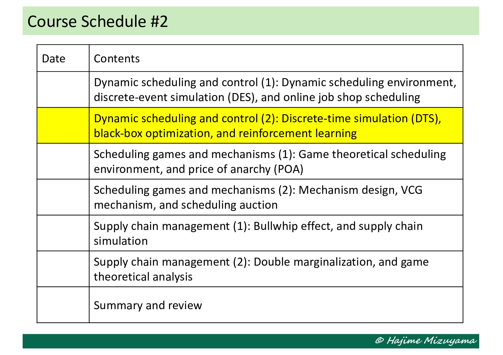
2. © Hajime Mizuyama Course Schedule #2 Date Contents Dynamic scheduling and control (1): Dynamic scheduling environment, discrete-event simulation (DES), and online job shop scheduling Dynamic scheduling and control (2): Discrete-time simulation (DTS), black-box optimization, and reinforcement learning Scheduling games and mechanisms (1): Game theoretical scheduling environment, and price of anarchy (POA) Scheduling games and mechanisms (2): Mechanism design, VCG mechanism, and scheduling auction Supply chain management (1): Bullwhip effect, and supply chain simulation Supply chain management (2): Double marginalization, and game theoretical analysis Summary and review
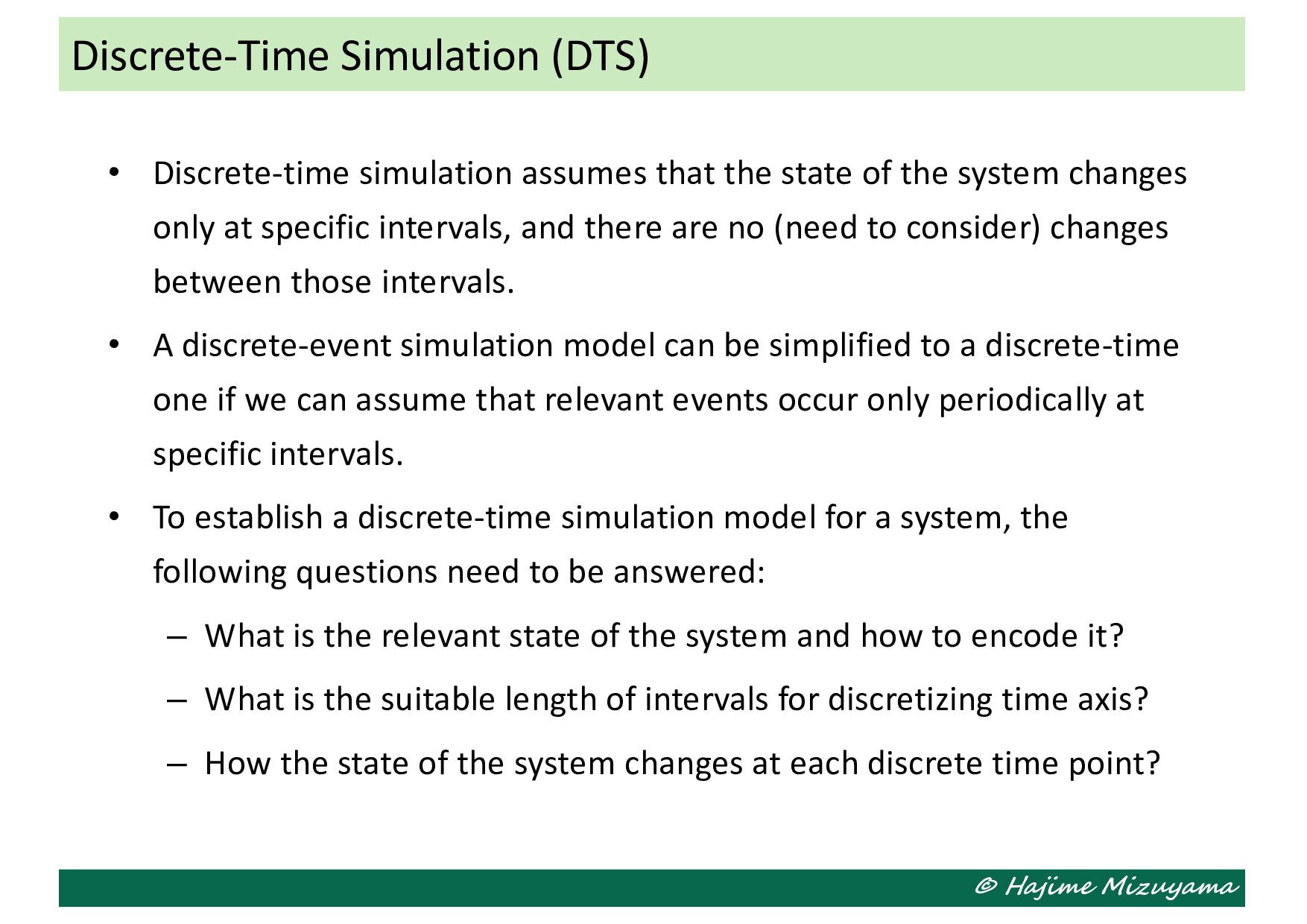
3. © Hajime Mizuyama • Discrete-time simulation assumes that the state of the system changes only at specific intervals, and there are no (need to consider) changes between those intervals. • A discrete-event simulation model can be simplified to a discrete-time one if we can assume that relevant events occur only periodically at specific intervals. • To establish a discrete-time simulation model for a system, the following questions need to be answered: – What is the relevant state of the system and how to encode it? – What is the suitable length of intervals for discretizing time axis? – How the state of the system changes at each discrete time point? Discrete-Time Simulation (DTS)
4. © Hajime Mizuyama 𝑠! ← Initial system state for 𝑡 = 1 to 𝑡"#$ do 𝑠% ← Resultant state updated at 𝑡 od General Algorithm for DTS
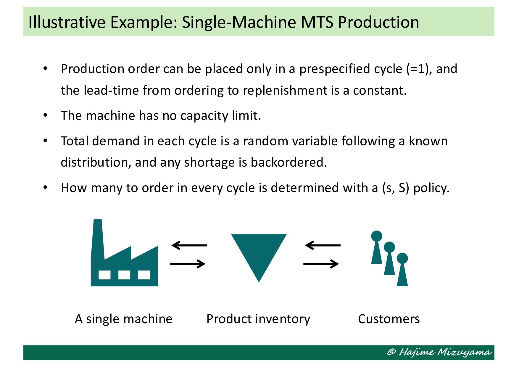
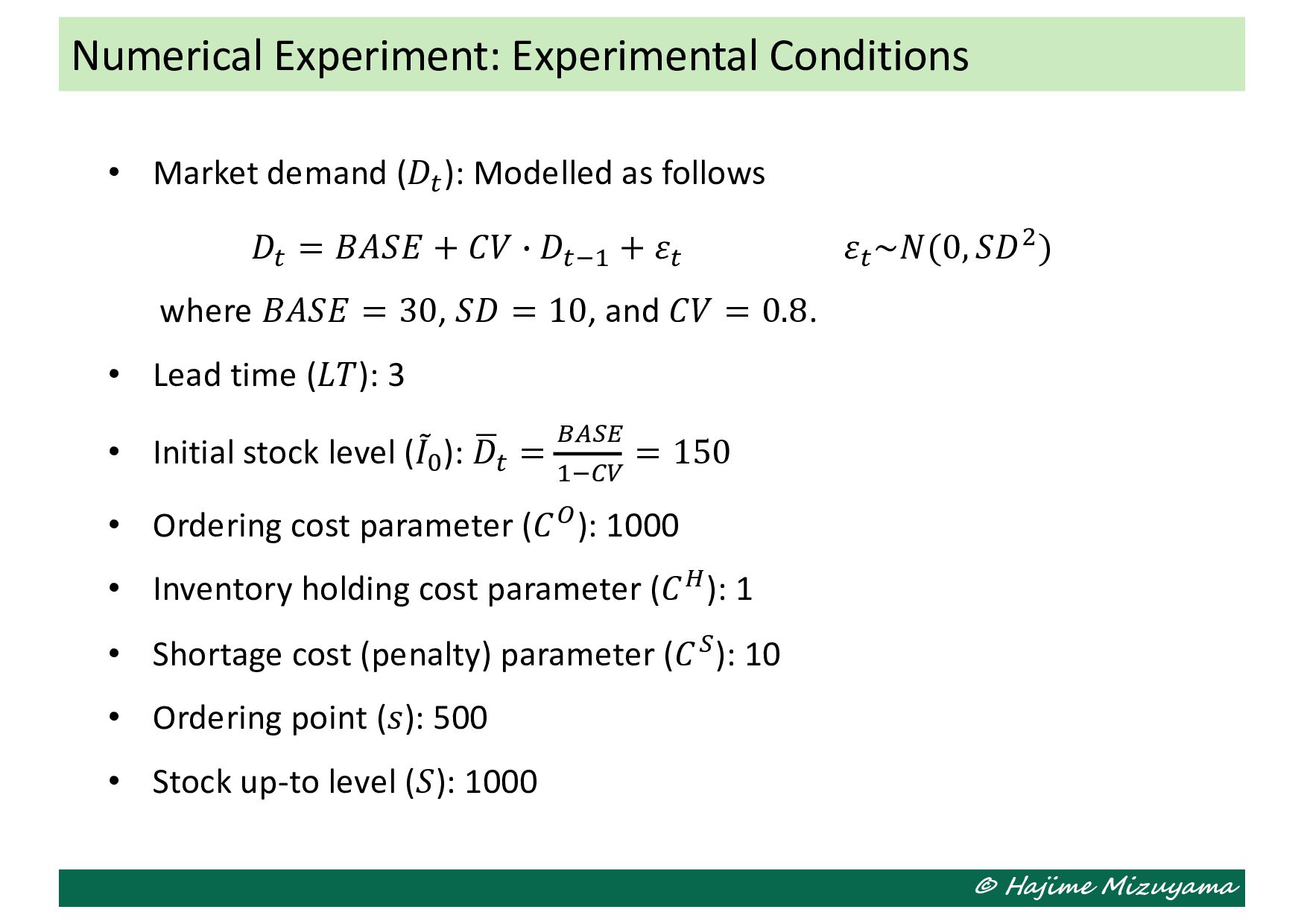
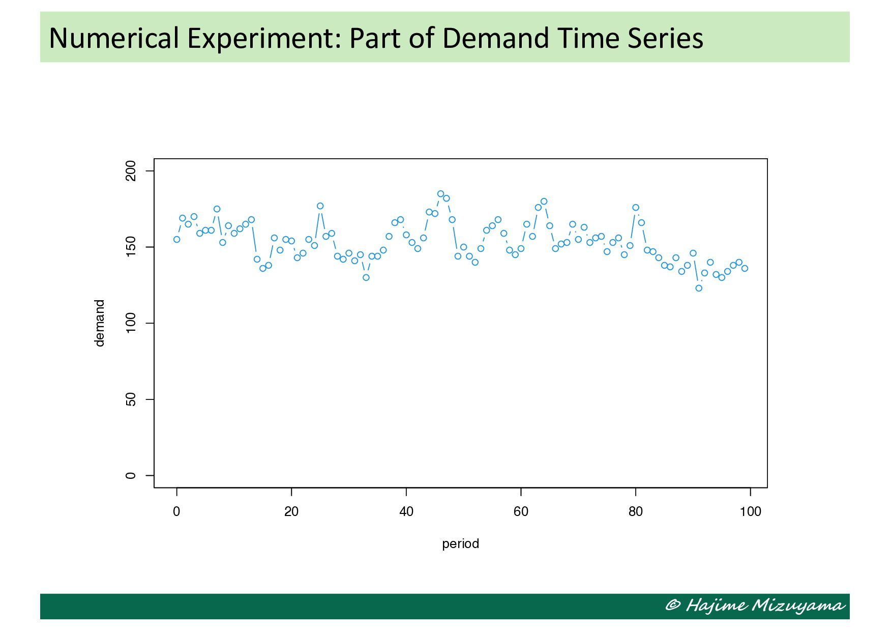
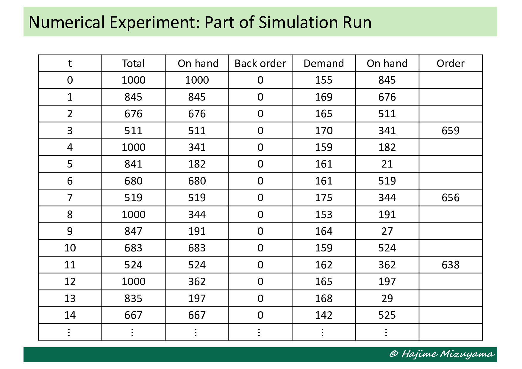
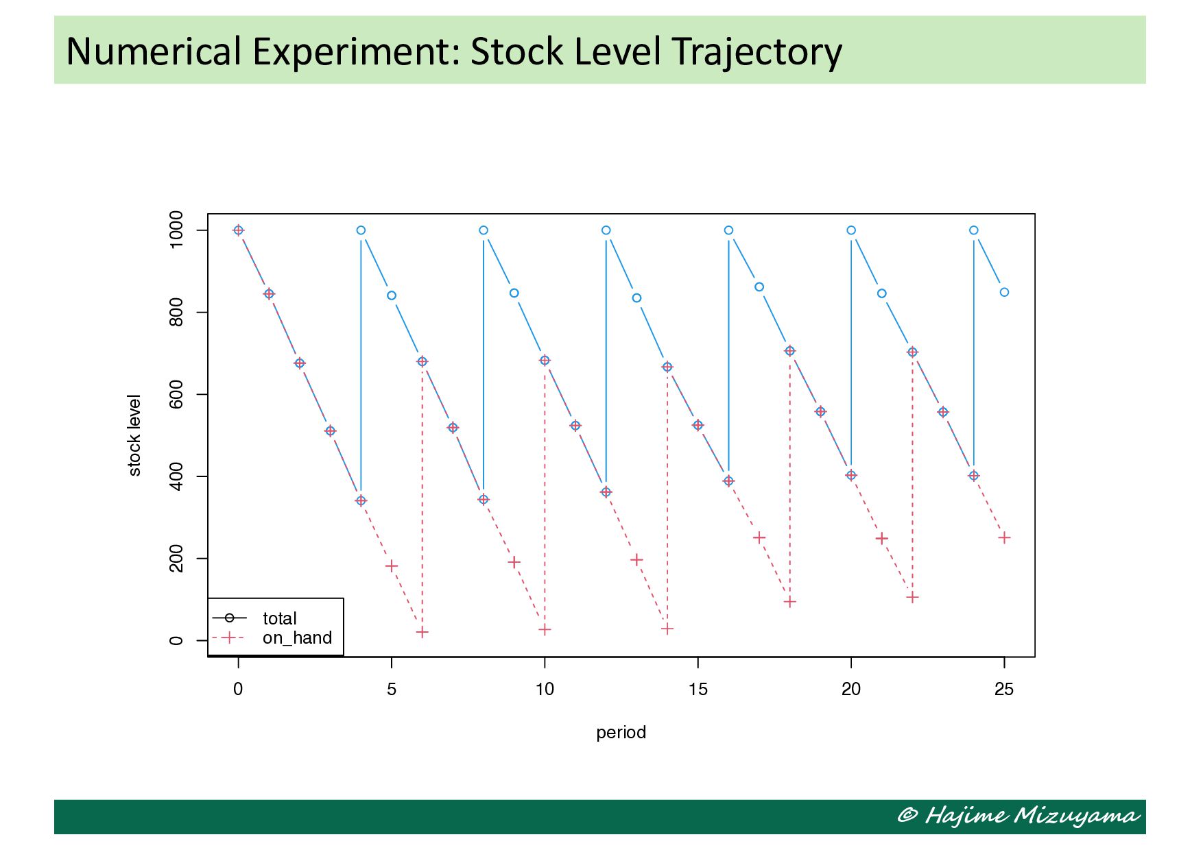
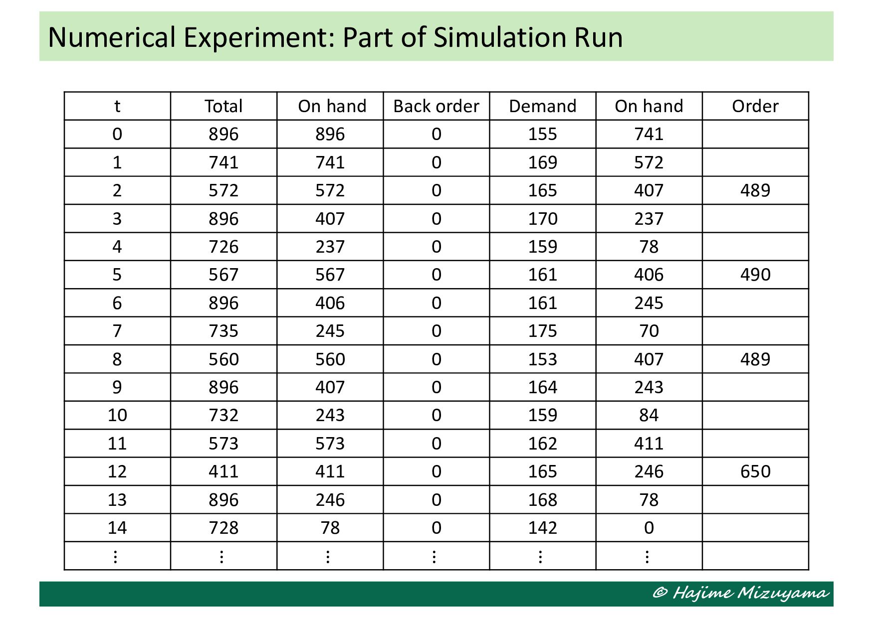
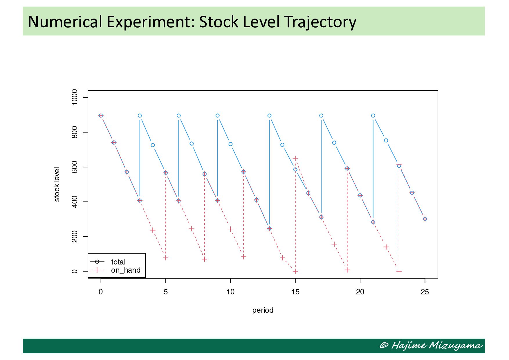
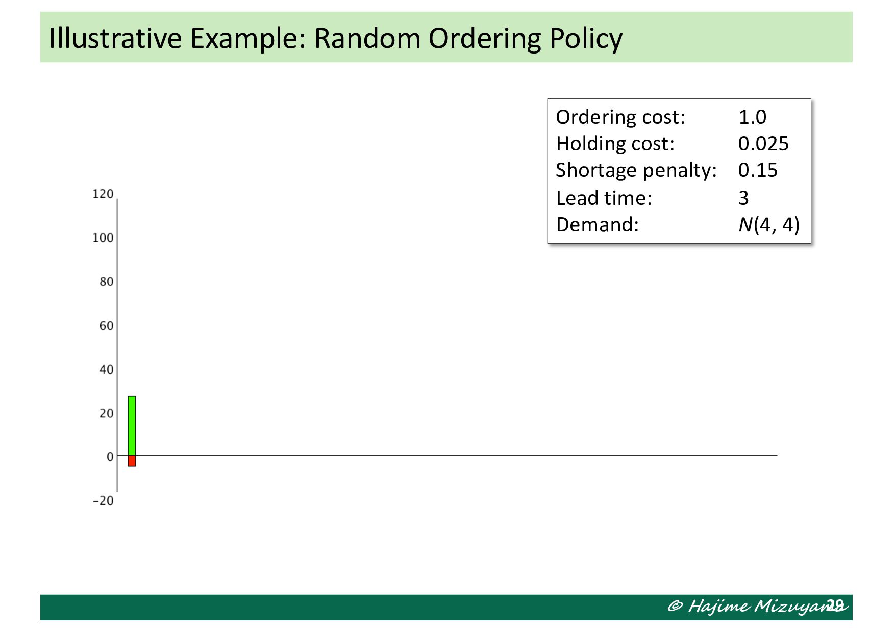
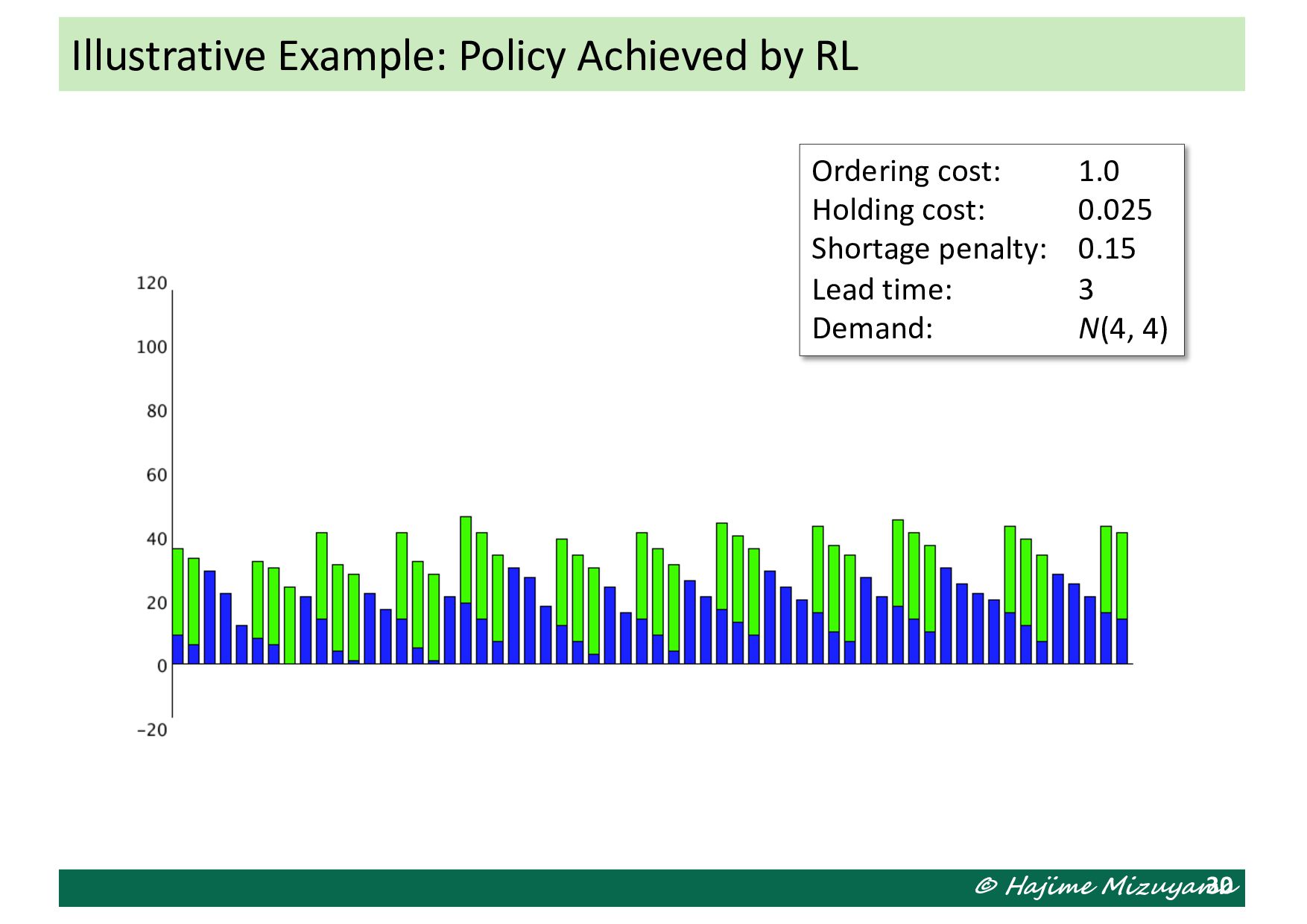
5. © Hajime Mizuyama • Production order can be placed only in a prespecified cycle (=1), and the lead-time from ordering to replenishment is a constant. • The machine has no capacity limit. • Total demand in each cycle is a random variable following a known distribution, and any shortage is backordered. • How many to order in every cycle is determined with a (s, S) policy. Illustrative Example: Single-Machine MTS Production A single machine Product inventory Customers
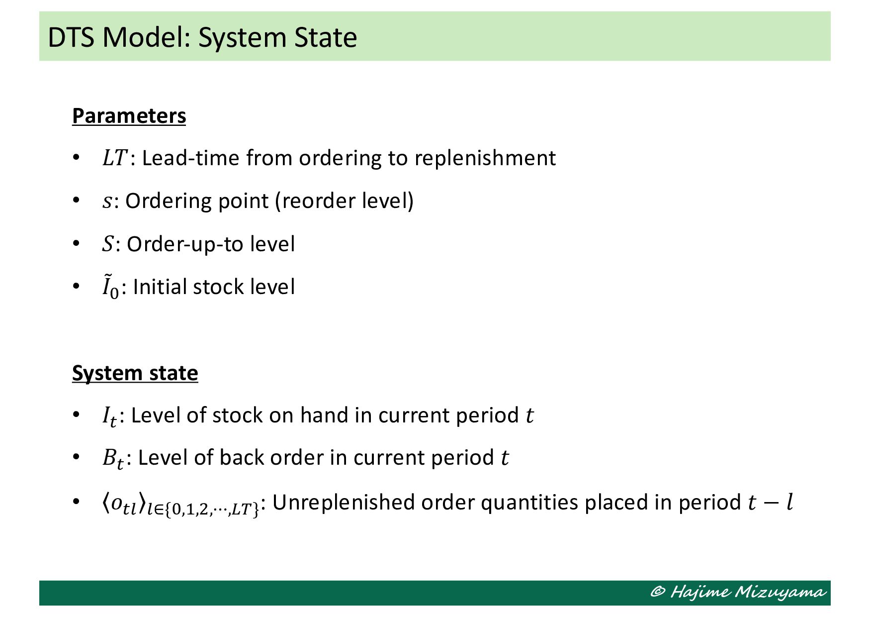
6. © Hajime Mizuyama Parameters • 𝐿𝑇: Lead-time from ordering to replenishment • 𝑠: Ordering point (reorder level) • 𝑆: Order-up-to level • ) 𝐼!: Initial stock level System state • 𝐼%: Level of stock on hand in current period 𝑡 • 𝐵%: Level of back order in current period 𝑡 • 𝑜%& &∈{!,*,+,⋯,-.}: Unreplenished order quantities placed in period 𝑡 − 𝑙 DTS Model: System State
7. © Hajime Mizuyama 𝐼! ← ) 𝐼!, 𝐵! ← 0, 𝑜!& ← 0 (∀𝑙 ∈ {0, 1, 2, ⋯ , 𝐿𝑇 − 1}) for 𝑡 = 1 to 𝑡"#$ do 𝑜%& ← 𝑜(%1*)(&1*) (∀𝑙 ∈ {1, 2, ⋯ , 𝐿𝑇}) 𝐷% ← Realized demand quantity in period 𝑡 𝐵% ← max(0, 𝐵%1* + 𝐷% − 𝐼%1* − 𝑜% -. ) 𝐼% ← max(0, 𝐼%1* + 𝑜% -. − 𝐵%1* − 𝐷% ) if 𝐼% − 𝐵% + ∑&3* -.1* 𝑜%& < 𝑠 then 𝑜%! ← 𝑆 − (𝐼% − 𝐵% + ∑&3* -.1* 𝑜%& ) else 𝑜%! ← 0 fi od DTS Model: Simulation Flow
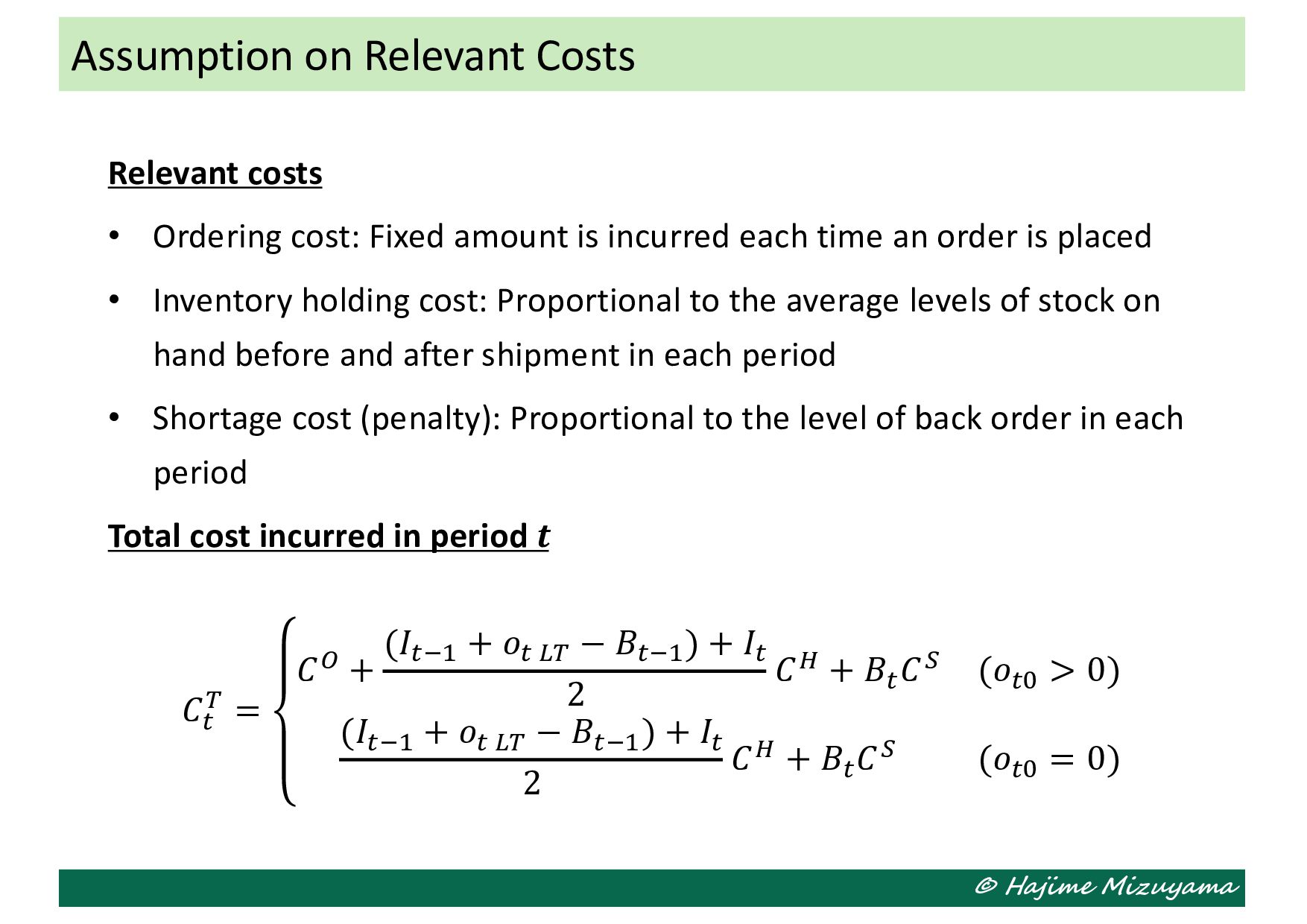
8. © Hajime Mizuyama Relevant costs • Ordering cost: Fixed amount is incurred each time an order is placed • Inventory holding cost: Proportional to the average levels of stock on hand before and after shipment in each period • Shortage cost (penalty): Proportional to the level of back order in each period Total cost incurred in period 𝒕 𝐶% . = 𝐶4 + (𝐼%1* + 𝑜% -. − 𝐵%1* ) + 𝐼% 2 𝐶5 + 𝐵% 𝐶6 (𝑜%! > 0) (𝐼%1* + 𝑜% -. − 𝐵%1* ) + 𝐼% 2 𝐶5 + 𝐵% 𝐶6 (𝑜%! = 0) Assumption on Relevant Costs
9. © Hajime Mizuyama • Market demand (𝐷%): Modelled as follows 𝐷% = 𝐵𝐴𝑆𝐸 + 𝐶𝑉 F 𝐷%1* + 𝜀% 𝜀% ~𝑁(0, 𝑆𝐷+) where 𝐵𝐴𝑆𝐸 = 30, 𝑆𝐷 = 10, and 𝐶𝑉 = 0.8. • Lead time (𝐿𝑇): 3 • Initial stock level () 𝐼!): M 𝐷% = 7869 *1:; = 150 • Ordering cost parameter (𝐶4): 1000 • Inventory holding cost parameter (𝐶5): 1 • Shortage cost (penalty) parameter (𝐶6): 10 • Ordering point (𝑠): 500 • Stock up-to level (𝑆): 1000 Numerical Experiment: Experimental Conditions
10. © Hajime Mizuyama 0 20 40 60 80 100 0 50 100 150 200 period demand Numerical Experiment: Part of Demand Time Series
11. © Hajime Mizuyama Numerical Experiment: Part of Simulation Run t Total On hand Back order Demand On hand Order 0 1000 1000 0 155 845 1 845 845 0 169 676 2 676 676 0 165 511 3 511 511 0 170 341 659 4 1000 341 0 159 182 5 841 182 0 161 21 6 680 680 0 161 519 7 519 519 0 175 344 656 8 1000 344 0 153 191 9 847 191 0 164 27 10 683 683 0 159 524 11 524 524 0 162 362 638 12 1000 362 0 165 197 13 835 197 0 168 29 14 667 667 0 142 525 ⋮ ⋮ ⋮ ⋮ ⋮ ⋮
12. © Hajime Mizuyama Numerical Experiment: Stock Level Trajectory 0 5 10 15 20 25 0 200 400 600 800 1000 period stock level total on_hand
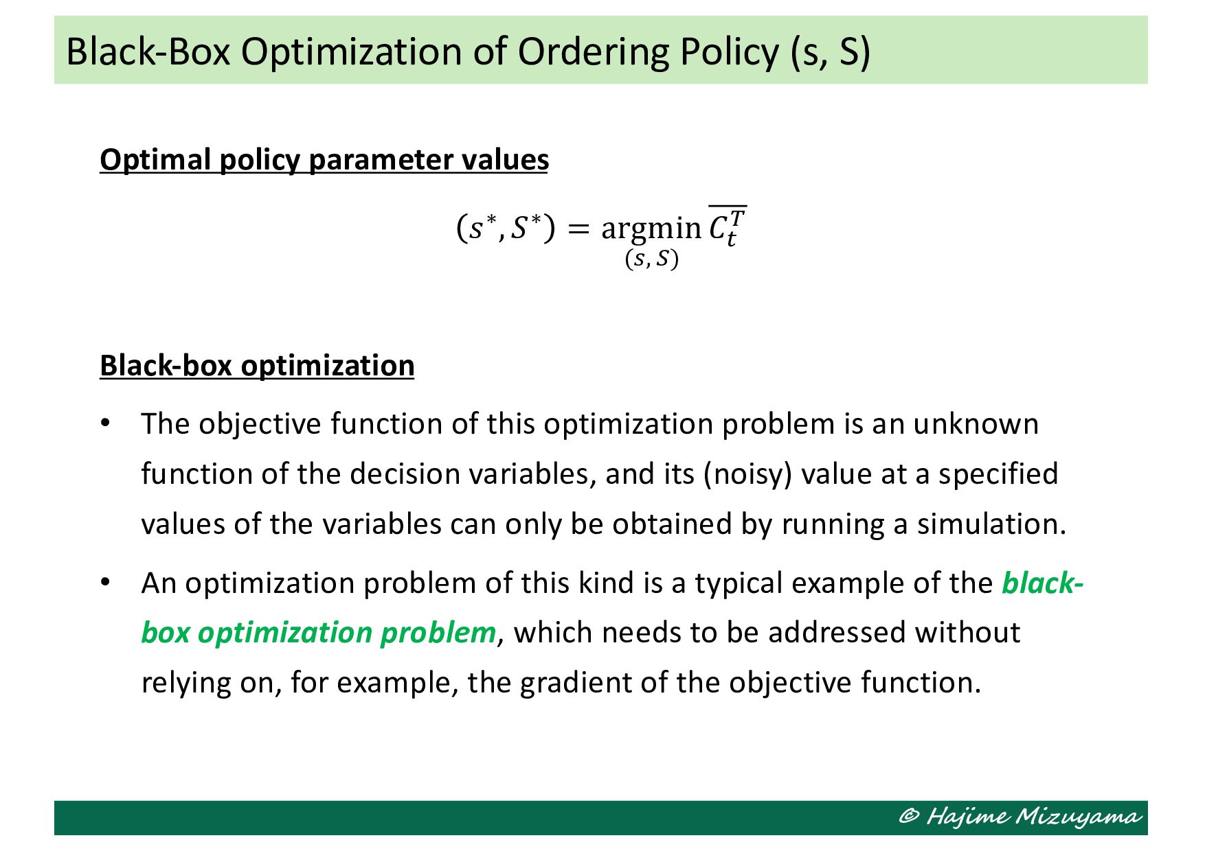
13. © Hajime Mizuyama Optimal policy parameter values 𝑠∗, 𝑆∗ = argmin (=, 6) 𝐶% . Black-box optimization • The objective function of this optimization problem is an unknown function of the decision variables, and its (noisy) value at a specified values of the variables can only be obtained by running a simulation. • An optimization problem of this kind is a typical example of the black- box optimization problem, which needs to be addressed without relying on, for example, the gradient of the objective function. Black-Box Optimization of Ordering Policy (s, S)
14. © Hajime Mizuyama 𝑥! ~ 𝑈 0, 1 "#$, 𝑣! ~ 𝑈 −1, 1 "#$, 𝑝! ← 𝑥! (∀𝑖 ∈ {1, ⋯ , Size}) 𝑝% ← argmin &!∈{&",⋯,&#$%&} 𝑓(𝑝! ) for 𝑙 = 1 to 𝐿$,- do for 𝑖 = 1 to Size do 𝑣!,. ← 𝑤𝑣!,. + 𝑐/ 𝑟/,. (𝑝!,. − 𝑥!,. ) + 𝑐0 𝑟0,. (𝑝. % − 𝑥!,. ) where 𝑟/,. , 𝑟0,. ∼ 𝑈(0, 1) (∀𝑑 ∈ {1, ⋯ , Dim}) 𝑥! ← 𝑥! + 𝑣! if 𝑓(𝑥! ) < 𝑓(𝑝! ) then 𝑝! ← 𝑥! fi if 𝑓(𝑥! ) < 𝑓(𝑝%) then 𝑝% ← 𝑥! fi od od Particle Swarm Optimization (PSO) for Minimizing 𝑓(𝑥) Dim: Dimension of 𝑥> Size: Particle size 𝑈(): Uniform distribution
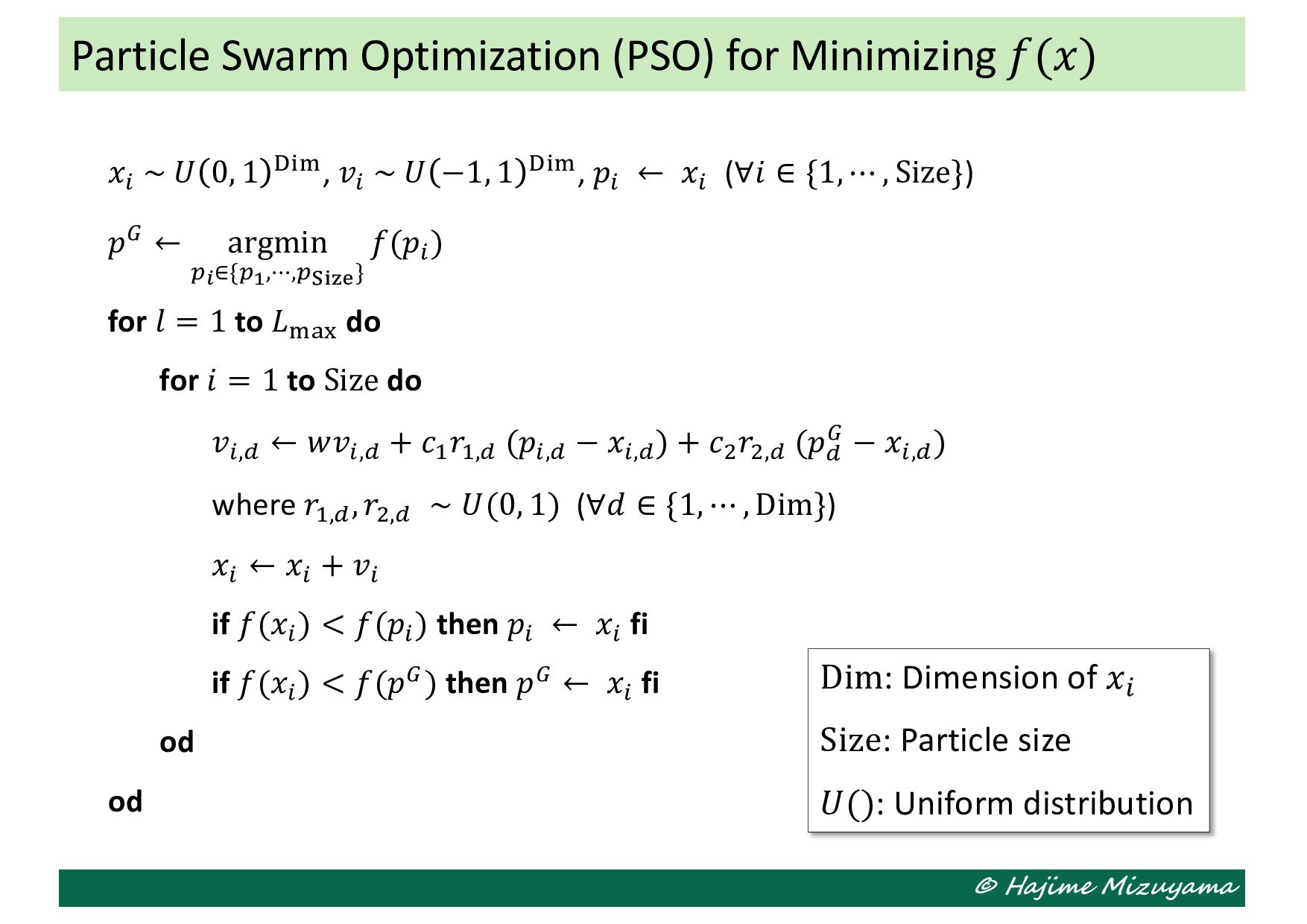
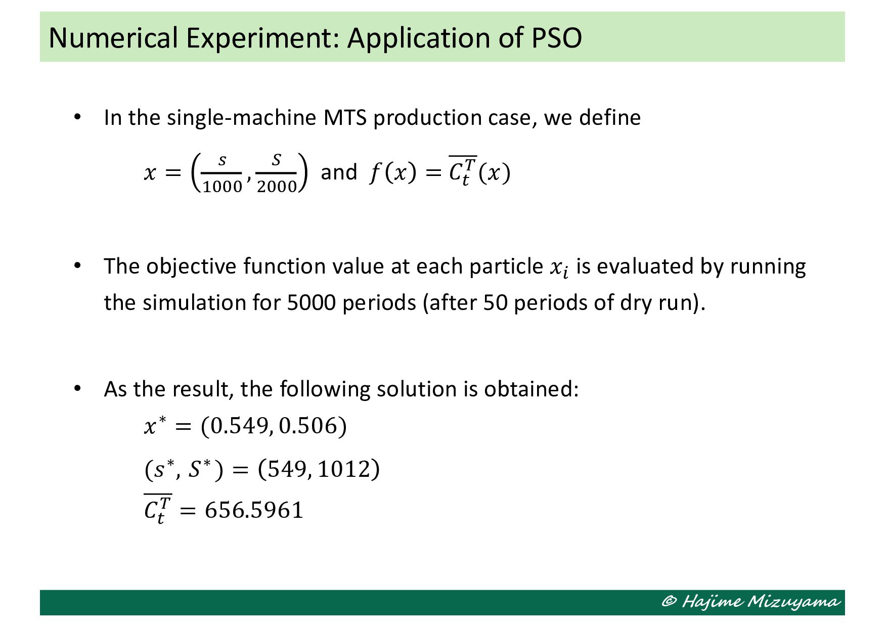
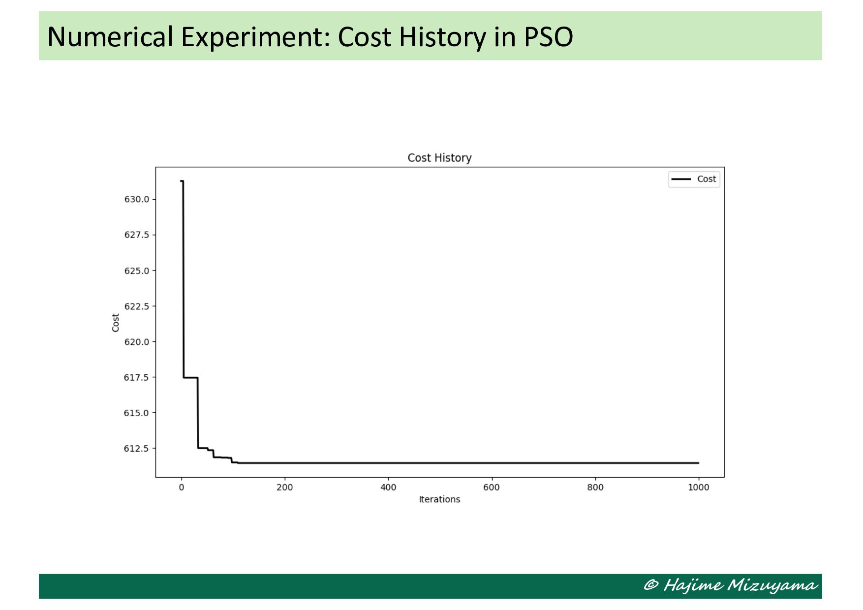
15. © Hajime Mizuyama • In the single-machine MTS production case, we define 𝑥 = = *!!! , 6 +!!! and 𝑓 𝑥 = 𝐶% .(𝑥) • The objective function value at each particle 𝑥> is evaluated by running the simulation for 5000 periods (after 50 periods of dry run). • As the result, the following solution is obtained: 𝑥∗ = (0.549, 0.506) (𝑠∗, 𝑆∗ ) = 549, 1012 𝐶% . = 656.5961 Numerical Experiment: Application of PSO
16. © Hajime Mizuyama Numerical Experiment: Cost History in PSO
17. © Hajime Mizuyama Numerical Experiment: Part of Simulation Run t Total On hand Back order Demand On hand Order 0 896 896 0 155 741 1 741 741 0 169 572 2 572 572 0 165 407 489 3 896 407 0 170 237 4 726 237 0 159 78 5 567 567 0 161 406 490 6 896 406 0 161 245 7 735 245 0 175 70 8 560 560 0 153 407 489 9 896 407 0 164 243 10 732 243 0 159 84 11 573 573 0 162 411 12 411 411 0 165 246 650 13 896 246 0 168 78 14 728 78 0 142 0 ⋮ ⋮ ⋮ ⋮ ⋮ ⋮
18. © Hajime Mizuyama Numerical Experiment: Stock Level Trajectory 0 5 10 15 20 25 0 200 400 600 800 1000 period stock level total on_hand
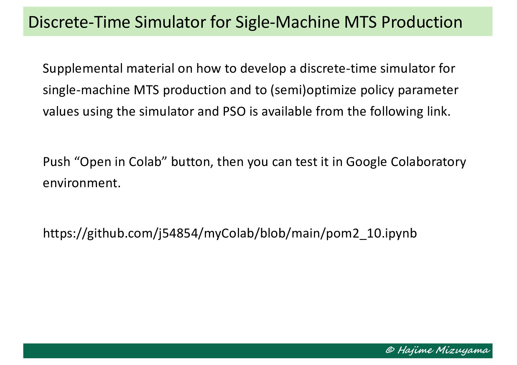
19. © Hajime Mizuyama Supplemental material on how to develop a discrete-time simulator for single-machine MTS production and to (semi)optimize policy parameter values using the simulator and PSO is available from the following link. Push “Open in Colab” button, then you can test it in Google Colaboratory environment. https://github.com/j54854/myColab/blob/main/pom2_10.ipynb Discrete-Time Simulator for Sigle-Machine MTS Production
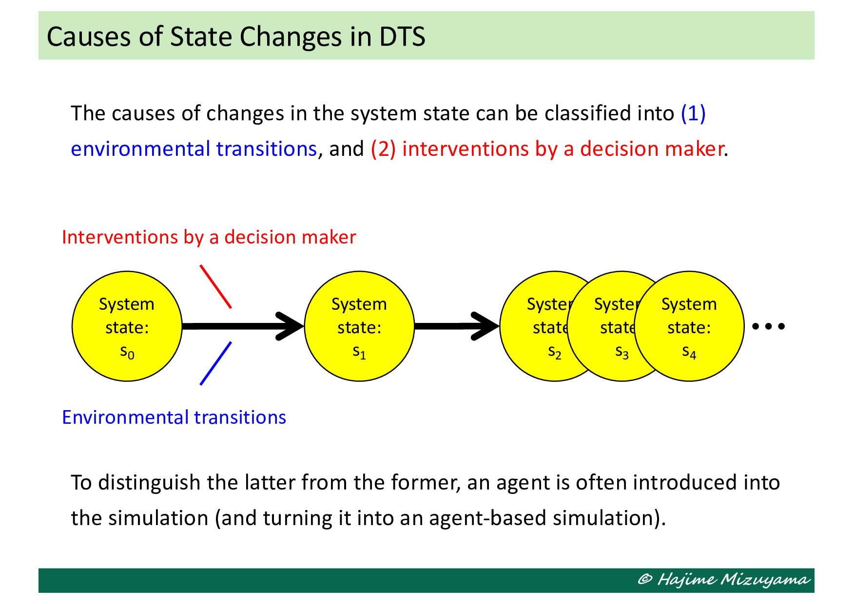
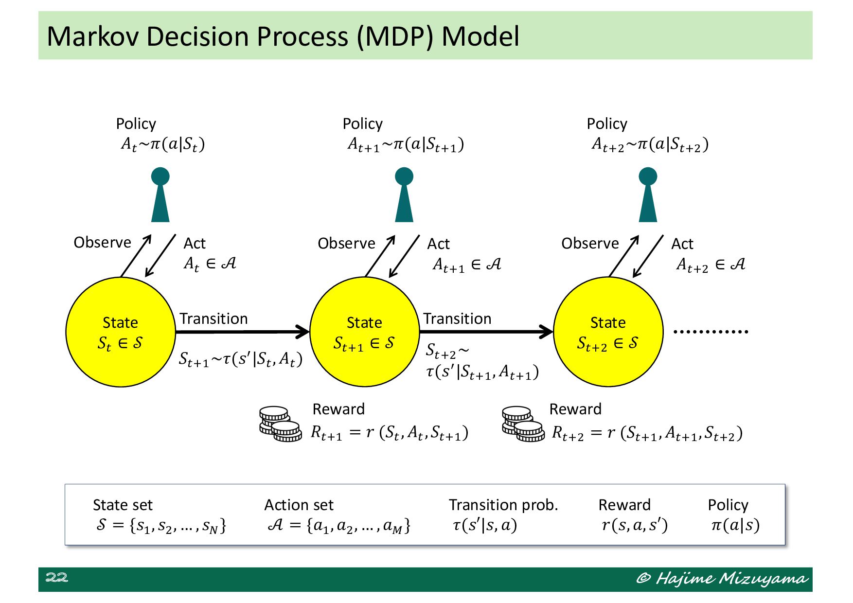
20. © Hajime Mizuyama The causes of changes in the system state can be classified into (1) environmental transitions, and (2) interventions by a decision maker. To distinguish the latter from the former, an agent is often introduced into the simulation (and turning it into an agent-based simulation). Causes of State Changes in DTS System state: s0 System state: s2 System state: s3 System state: s4 System state: s1 Environmental transitions Interventions by a decision maker
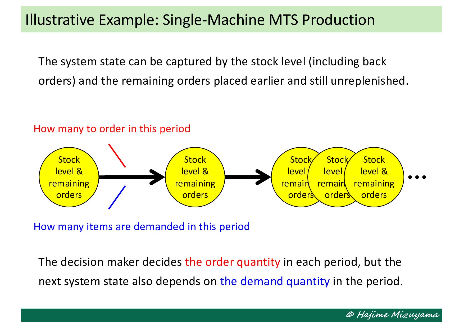
21. © Hajime Mizuyama The system state can be captured by the stock level (including back orders) and the remaining orders placed earlier and still unreplenished. The decision maker decides the order quantity in each period, but the next system state also depends on the demand quantity in the period. Illustrative Example: Single-Machine MTS Production Stock level & remaining orders Stock level & remaining orders Stock level & remaining orders Stock level & remaining orders Stock level & remaining orders How many items are demanded in this period How many to order in this period
22. © Hajime Mizuyama Markov Decision Process (MDP) Model 22 State 𝑆! ∈ 𝒮 Observe Act 𝐴! ∈ 𝒜 State set 𝒮 = {𝑠" , 𝑠# , … , 𝑠$ } Action set 𝒜 = {𝑎" , 𝑎# , … , 𝑎% } Transition prob. 𝜏(𝑠′|𝑠, 𝑎) Reward 𝑟(𝑠, 𝑎, 𝑠′) Policy 𝐴! ~𝜋(𝑎|𝑆! ) Observe Act 𝐴!&" ∈ 𝒜 Policy 𝐴!&" ~𝜋(𝑎|𝑆!&" ) Observe Act 𝐴!&# ∈ 𝒜 Policy 𝐴!&# ~𝜋(𝑎|𝑆!&# ) State 𝑆!&" ∈ 𝒮 𝑆!&" ~𝜏(𝑠'|𝑆! , 𝐴! ) 𝑅!&" = 𝑟 (𝑆! , 𝐴! , 𝑆!&" ) Transition Reward State 𝑆!&# ∈ 𝒮 𝑆!&# ~ 𝜏(𝑠'|𝑆!&" , 𝐴!&" ) 𝑅!&# = 𝑟 (𝑆!&" , 𝐴!&" , 𝑆!&# ) Transition Reward Policy 𝜋(𝑎|𝑠)
23. © Hajime Mizuyama Value Functions and Q-Learning State value function (discounted sum of rewards obtained from now on) 𝑉 N 𝑠 = 𝔼N [𝑅%O* + 𝛾 F 𝑅%O+ + 𝛾+ F 𝑅%OP + ⋯ |𝑆% = 𝑠] = 𝔼N [𝑅%O* + 𝛾 F 𝑉 N (𝑆%O* )|𝑆% = 𝑠] Action value function (Q-table/Q-function) 𝑄 𝑠, 𝑎 = 𝔼N [𝑅%O* + 𝛾 F 𝑅%O+ + 𝛾+ F 𝑅%OP + ⋯ |𝑆% = 𝑠, 𝐴% = 𝑎] = 𝔼N [𝑅%O* + 𝛾 F max QR 𝑄 (𝑆%O* , 𝑎′) |𝑆% = 𝑠, 𝐴% = 𝑎] Q-learning Refine approximated Q values step by step through simulation by: 𝑄 𝑆% , 𝐴% ← (1 − 𝛼) F 𝑄 𝑆% , 𝐴% + 𝛼 F [𝑅%O* + 𝛾 F max QR 𝑄 𝑆%O* , 𝑎R ] 23
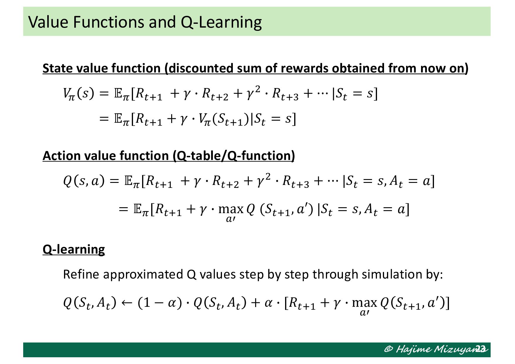
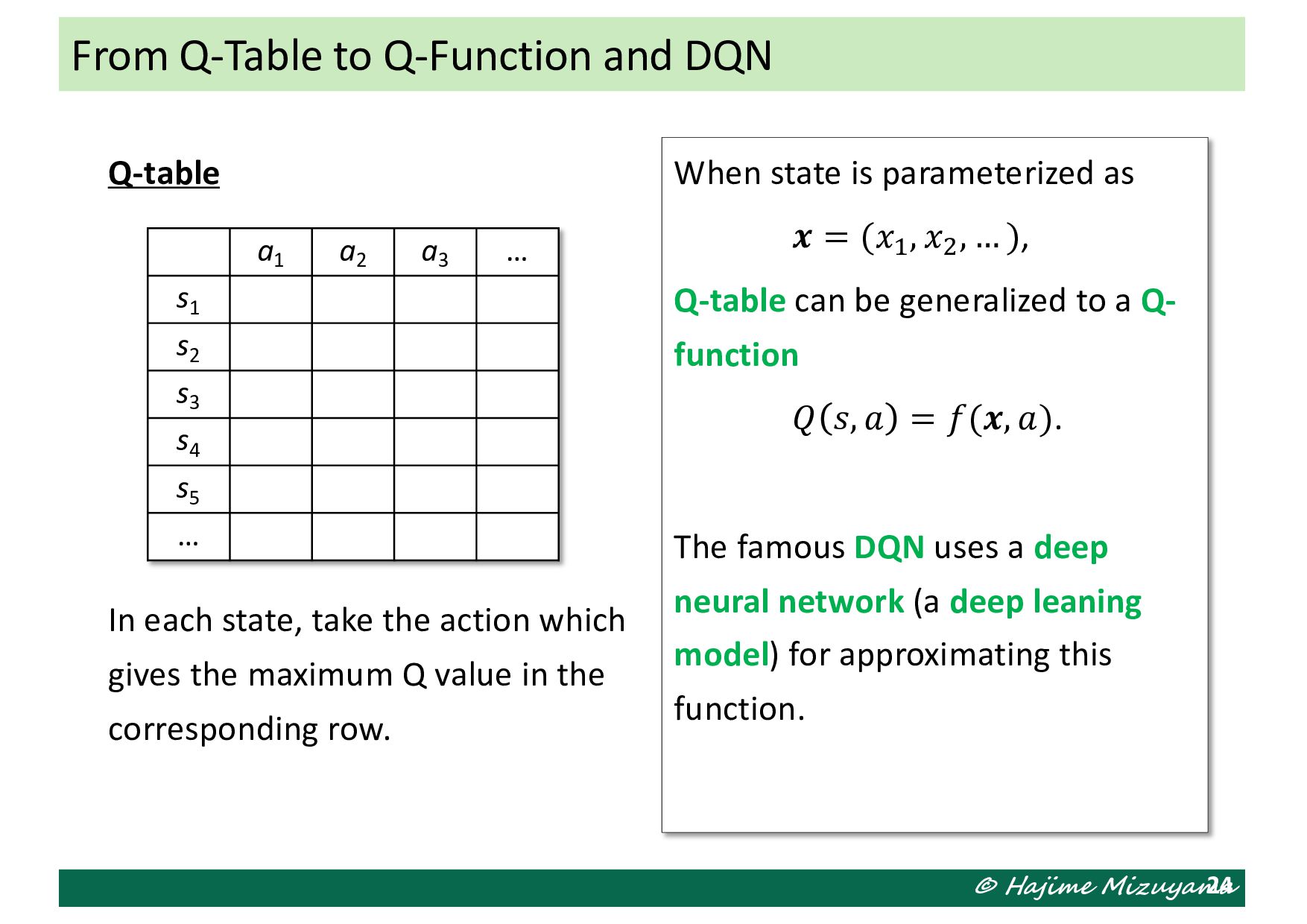
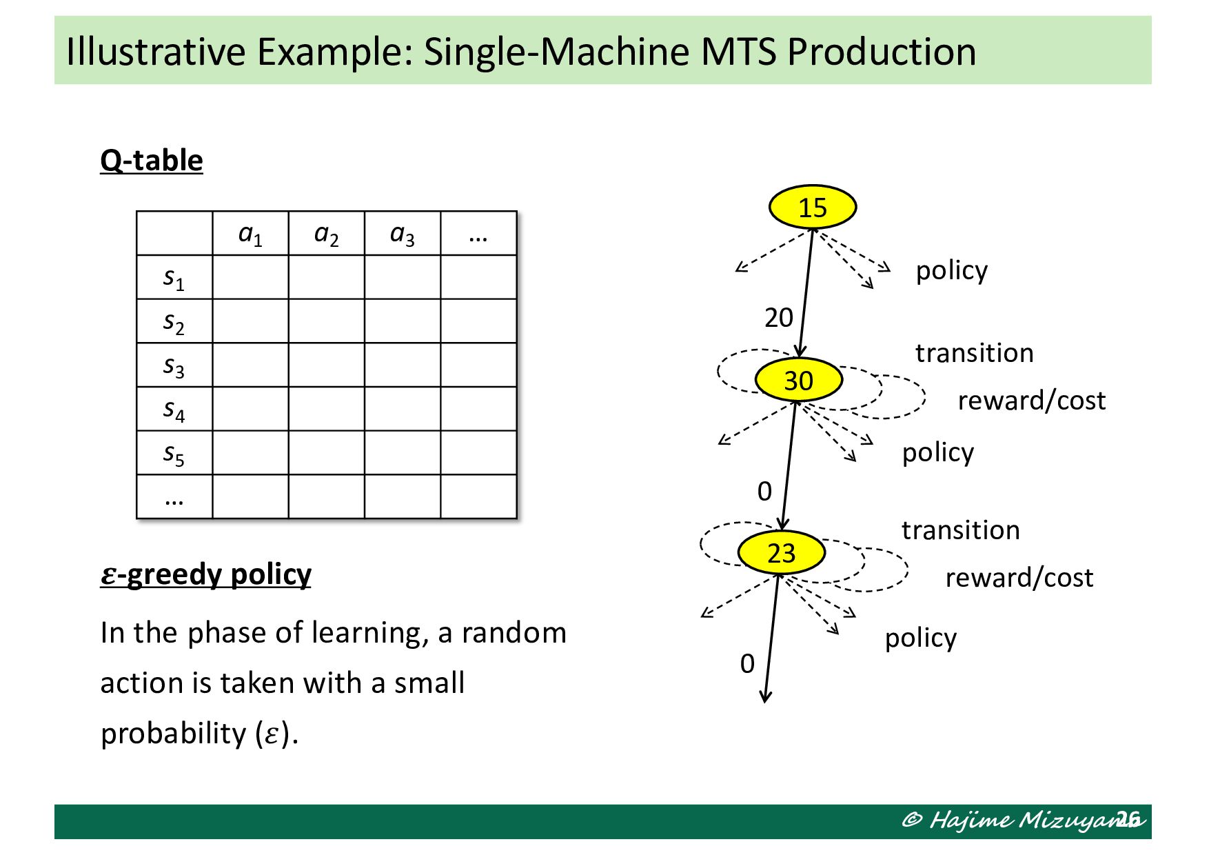
24. © Hajime Mizuyama From Q-Table to Q-Function and DQN Q-table In each state, take the action which gives the maximum Q value in the corresponding row. When state is parameterized as 𝒙 = (𝑥* , 𝑥+ , … ), Q-table can be generalized to a Q- function 𝑄 𝑠, 𝑎 = 𝑓(𝒙, 𝑎). The famous DQN uses a deep neural network (a deep leaning model) for approximating this function. 24 a1 a2 a3 … s1 s2 s3 s4 s5 …
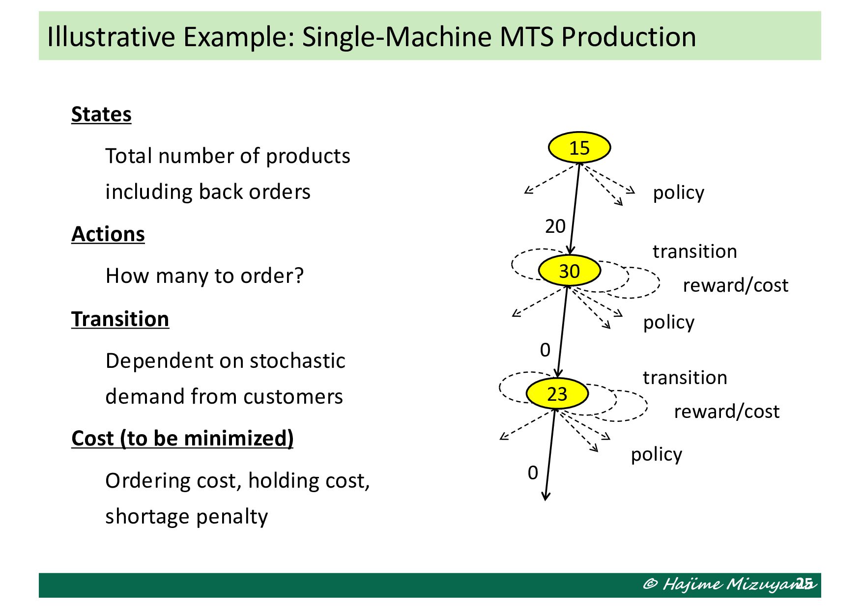
25. © Hajime Mizuyama Illustrative Example: Single-Machine MTS Production States Total number of products including back orders Actions How many to order? Transition Dependent on stochastic demand from customers Cost (to be minimized) Ordering cost, holding cost, shortage penalty 25 15 20 policy 30 transition reward/cost 0 policy 23 transition reward/cost 0 policy
26. © Hajime Mizuyama Illustrative Example: Single-Machine MTS Production Q-table 𝜺-greedy policy In the phase of learning, a random action is taken with a small probability (𝜀). 26 a1 a2 a3 … s1 s2 s3 s4 s5 … 15 20 policy 30 transition reward/cost 0 policy 23 transition reward/cost 0 policy
27. © Hajime Mizuyama Illustrative Example: How Q-Table is Updated through Learning 27
28. © Hajime Mizuyama Illustrative Example: Cost Reduction through Learning 28 Ordering cost: 1.0 Holding cost: 0.025 Shortage penalty: 0.15 Lead time: 3 Demand: N(4, 4)
29. © Hajime Mizuyama Illustrative Example: Random Ordering Policy 29 Ordering cost: 1.0 Holding cost: 0.025 Shortage penalty: 0.15 Lead time: 3 Demand: N(4, 4)
30. © Hajime Mizuyama Illustrative Example: Policy Achieved by RL 30 Ordering cost: 1.0 Holding cost: 0.025 Shortage penalty: 0.15 Lead time: 3 Demand: N(4, 4)