IMSI Short Talk 2025-04-10

Informal talk given at the NSF-funded Institute for Mathematical and Statistical Innovation (IMSI) as part of the long program on Uncertainty Quantification and AI for Complex Systems

Transcript

1. Fred J. Hickernell, Illinois Institute of Technology April 10, 2025 Data-Driven Error Bounds for Monte Carlo Thanks to • Lulu Kang, Devon Lin, and IMSI • My collaborators • US National Science Foundation #2316011 Slides at speakerdeck.com/fjhickernell/imsi-short-talk-2025-04-10
4. Next 25 minutes
5. Next 25 minutes • What must you assume to obtain driven error bounds?
6. Next 25 minutes • What must you assume to obtain driven error bounds? • approach
7. Next 25 minutes • What must you assume to obtain driven error bounds? • approach • approach
8. Next 25 minutes • What must you assume to obtain driven error bounds? • approach • approach • IID Monte Carlo
9. Next 25 minutes • What must you assume to obtain driven error bounds? • approach • approach • IID Monte Carlo • Quasi-Monte Carlo
10. Next 25 minutes • What must you assume to obtain driven error bounds? • approach • approach • IID Monte Carlo • Quasi-Monte Carlo • Discussion and future work
11. Monte Carlo
12. Monte Carlo • You want to know some property of a random variable, , e.g., mean, probability density, or quartile Y
13. Monte Carlo • You want to know some property of a random variable, , e.g., mean, probability density, or quartile Y • You generate samples , which you use to approximate the property of Y1 , Y2 , . . . , Yn Y
14. Monte Carlo • You want to know some property of a random variable, , e.g., mean, probability density, or quartile Y • You generate samples , which you use to approximate the property of Y1 , Y2 , . . . , Yn Y • How do you generate samples? • How do you approximate the mean, density, quartile, etc.? • How many samples do you need and/or what error bound can you con fi dently assert?
15. Examples of Monte Carlo Y = f(X), X ∈ ℝd and is easy to sample Y = f(X) = option payo ff underground water pressure with random rock porosity pixel intensity from random ray option price average water pressure average pixel intensity = μ := 𝔼 (Y) may be dozens or hundreds d
16. IID Monte Carlo Confidence Intervals
17. • Monte Carlo approximates 
 
 by , for μ := 𝔼 (Y) = 𝔼 [f( X ⏟ ∼ 𝒰 [0,1]d )] = ∫ [0,1]d f(x) dx ̂ μn := 1 n n ∑ i=1 f(xi ) {xi }n i=1 IID ∼ 𝒰 [0,1]d IID Monte Carlo Confidence Intervals
18. • Monte Carlo approximates 
 
 by , for μ := 𝔼 (Y) = 𝔼 [f( X ⏟ ∼ 𝒰 [0,1]d )] = ∫ [0,1]d f(x) dx ̂ μn := 1 n n ∑ i=1 f(xi ) {xi }n i=1 IID ∼ 𝒰 [0,1]d • Chebyshev: for ℙ[|μ − ̂ μn | ≤ σ/ αn] ≥ 1 − α f ∈ {f : Std(f ) ≤ σ} IID Monte Carlo Confidence Intervals
19. • Monte Carlo approximates 
 
 by , for μ := 𝔼 (Y) = 𝔼 [f( X ⏟ ∼ 𝒰 [0,1]d )] = ∫ [0,1]d f(x) dx ̂ μn := 1 n n ∑ i=1 f(xi ) {xi }n i=1 IID ∼ 𝒰 [0,1]d • Chebyshev: for ℙ[|μ − ̂ μn | ≤ σ/ αn] ≥ 1 − α f ∈ {f : Std(f ) ≤ σ} • Empirical Bernstein [MP09]: for , where is the sample variance ℙ [ |μ − ̂ μn | ≤ 2 ̂ σ2 n log(4/α) n + 7 log(4/α) 3(n − 1) ] ≥ 1 − α f = {f ∈ ℒ2[0,1]d : 0 ≤ f(x) ≤ 1} ̂ σ2 n • See [WSR24] for betting con fi dence intervals IID Monte Carlo Confidence Intervals
20. IID Monte Carlo Confidence Intervals
21. • Monte Carlo approximates 
 
 by , for μ := 𝔼 (Y) = 𝔼 [f( X ⏟ ∼ 𝒰 [0,1]d )] = ∫ [0,1]d f(x) dx ̂ μn := 1 n n ∑ i=1 f(xi ) {xi }n i=1 IID ∼ 𝒰 [0,1]d IID Monte Carlo Confidence Intervals
22. • Monte Carlo approximates 
 
 by , for μ := 𝔼 (Y) = 𝔼 [f( X ⏟ ∼ 𝒰 [0,1]d )] = ∫ [0,1]d f(x) dx ̂ μn := 1 n n ∑ i=1 f(xi ) {xi }n i=1 IID ∼ 𝒰 [0,1]d • Central Limit Theorem: Compute the sample standard deviation, , 
 for of nice functions
 ̂ σnσ ℙ[ |μ − ̂ μn | ≤ 1.96 fdg(n) ̂ σnσ / n ] ≥ 95 % f ∈ IID Monte Carlo Confidence Intervals
23. • Monte Carlo approximates 
 
 by , for μ := 𝔼 (Y) = 𝔼 [f( X ⏟ ∼ 𝒰 [0,1]d )] = ∫ [0,1]d f(x) dx ̂ μn := 1 n n ∑ i=1 f(xi ) {xi }n i=1 IID ∼ 𝒰 [0,1]d • Central Limit Theorem: Compute the sample standard deviation, , 
 for of nice functions
 ̂ σnσ ℙ[ |μ − ̂ μn | ≤ 1.96 fdg(n) ̂ σnσ / n ] ≥ 95 % f ∈ • [HJLO13] gives a rigorous approach using Berry-Esseen inequalities IID Monte Carlo Confidence Intervals
24. • Monte Carlo approximates 
 
 by , for μ := 𝔼 (Y) = 𝔼 [f( X ⏟ ∼ 𝒰 [0,1]d )] = ∫ [0,1]d f(x) dx ̂ μn := 1 n n ∑ i=1 f(xi ) {xi }n i=1 IID ∼ 𝒰 [0,1]d • Central Limit Theorem: Compute the sample standard deviation, , 
 for of nice functions
 ̂ σnσ ℙ[ |μ − ̂ μn | ≤ 1.96 fdg(n) ̂ σnσ / n ] ≥ 95 % f ∈ • [HJLO13] gives a rigorous approach using Berry-Esseen inequalities • Bahadur and Savage [BS56] explain why the cone should be non-convex IID Monte Carlo Confidence Intervals
25. Low discrepancy (LD) sequences can beat grids and IID for moderate to large d Quasi-Monte Carlo (QMC) methods [HKS25] 0.00 0.25 0.50 0.75 1.00 xi1 0.00 0.25 0.50 0.75 1.00 xi2 64 IID points for d = 6 0.0 0.2 0.4 0.6 0.8 1.0 xi1 0.0 0.2 0.4 0.6 0.8 1.0 xi2 64 Grid Points for d =6 0.00 0.25 0.50 0.75 1.00 xi1 0.00 0.25 0.50 0.75 1.00 xi2 64 Sobol’ points for d = 6 0.00 0.25 0.50 0.75 1.00 xi1 0.00 0.25 0.50 0.75 1.00 xi2 64 Lattice Points for d = 6
26. Low discrepancy (LD) sequences can beat grids and IID for moderate to large d Quasi-Monte Carlo methods 100 101 102 103 104 105 106 107 Sample Size, n 10°6 10°4 10°2 100 Relative Error, |(µ ° ˆ µn )/µ| grid O(n°1/5) IID MC med O(n°1/2) LD med O(n°1) μ = ∫ ℝ6 cos(∥x∥) exp( −∥x∥2) dx [Kei96]
27. Discrepancy measures the quality of [H00] x0 , x1 , … μ := expectation 𝔼 [f( X ⏟ ∼ 𝒰 ([0,1]d) )] = integral ∫ [0,1]d f(x) dx ≈ sample mean 1 n n ∑ i=1 f(xi ) =: ̂ μn |μ − ̂ μn | ≤ tight discrepancy({xi }n i=1 ) norm of the error functional variation(f ) semi-norm
28. Discrepancy measures the quality of [H00] x0 , x1 , … μ := expectation 𝔼 [f( X ⏟ ∼ 𝒰 ([0,1]d) )] = integral ∫ [0,1]d f(x) dx ≈ sample mean 1 n n ∑ i=1 f(xi ) =: ̂ μn |μ − ̂ μn | ≤ tight discrepancy({xi }n i=1 ) norm of the error functional variation(f ) semi-norm If is in a Hilbert space with reproducing kernel , then f ℋ K discrepancy2({xi }n i=1 ) = ∫ [0,1]d×[0,1]d K(t, x) dt dx − 2 n n ∑ i=1 ∫ [0,1]d K(t, xi ) dt + 1 n2 n ∑ i,j=1 K(xi , xj ) variation(f ) = inf c∈ℝ ∥f − c∥ℋ operations 𝒪 (dn2) infeasible to compute
29. Deterministic stopping rules for QMC [HJ16, JH16, SJ24] μ := expectation 𝔼 [f( X ⏟ ∼ 𝒰 ([0,1]d) )] = integral ∫ [0,1]d f(x) dx ≈ sample mean 1 n n ∑ i=1 f(xi ) =: ̂ μn , want |μ − ̂ μn | ≤ ε • For lattices, , , • due to aliasing ( constant for all ) • Assume that lies in of functions whose Fourier coe ffi cients decay reasonably • Approximate by a one-dimensional FFT of • FFT approximations provide a rigorous data-driven bound on with work • Similarly for digital nets ̂ f(k) := ∫ [0,1]d f(x) 𝖾 −2π −1kT x dx f(x) = ∑ k∈ℤd ̂ f(k) 𝖾 2π −1kT x μ = ̂ f(0) μ − ̂ μn 𝖾 2π −1kT xi i f ̂ f(k) {f(xi )}n−1 i=0 μ − ̂ μn 𝒪 (n log n)
30. Deterministic stopping rules for QMC [HJ16, JH16, SJ24] μ := expectation 𝔼 [f( X ⏟ ∼ 𝒰 ([0,1]d) )] = integral ∫ [0,1]d f(x) dx ≈ sample mean 1 n n ∑ i=1 f(xi ) =: ̂ μn , want |μ − ̂ μn | ≤ ε • For lattices, , , • due to aliasing ( constant for all ) • Assume that lies in of functions whose Fourier coe ffi cients decay reasonably • Approximate by a one-dimensional FFT of • FFT approximations provide a rigorous data-driven bound on with work • Similarly for digital nets ̂ f(k) := ∫ [0,1]d f(x) 𝖾 −2π −1kT x dx f(x) = ∑ k∈ℤd ̂ f(k) 𝖾 2π −1kT x μ = ̂ f(0) μ − ̂ μn 𝖾 2π −1kT xi i f ̂ f(k) {f(xi )}n−1 i=0 μ − ̂ μn 𝒪 (n log n)
31. Bayesian stopping rules for QMC [JH19, JH22] μ := expectation 𝔼 [f( X ⏟ ∼ 𝒰 ([0,1]d) )] = integral ∫ [0,1]d f(x) dx ≈ sample mean 1 n n ∑ i=1 f(xi ) =: ̂ μn , want |μ − ̂ μn | ≤ ε • Assume is a Gaussian stochastic process with covariance kernel , where the hyper-parameters are properly tuned • Construct a Bayesian credible interval for • If is chosen to fi t the lattice/digital sequences, then the computation normally required reduces to • Works for in f K μ K 𝒪 (n3) 𝒪 (n log n) f
32. Keister example sample size and time μ = ∫ ℝ6 cos(∥x∥) exp( −∥x∥2) dx [Kei96] 10°4 10°3 10°2 10°1 Relative error tolerance, " 102 103 104 105 106 107 Sample size, n Sobol’ deterministic lattice deterministic Sobol’ Bayesian lattice Bayesian 10°4 10°3 10°2 10°1 Relative error tolerance, " 10°4 10°3 10°2 10°1 100 101 Computation time (sec) Sobol’ deterministic lattice deterministic Sobol’ Bayesian lattice Bayesian
33. Discussion and future work Adaptive 1-D Integration Adaptive (quasi-)Monte Carlo Adaptive multi-level (quasi-)Monte Carlo Adaptive FEM for PDEs w/ a posteriori error bounds Adaptive multi-level (quasi-)Monte Carlo with FEM for PDEs with randomness • For replications of QMC for bounded see [JO25] • For another view, see [LENOT24] f
34. MCM2025Chicago.org July 28 – August 1 Plenary Speakers Nicholas Chopin, ENSAE Peter Glynn, Stanford U
 Roshan Joseph, Georgia Tech Christiane Lemieux, U Waterloo
 Matt Pharr, NVIDIA Veronika Rockova, U Chicago
 Uros Seljak, U California, Berkeley Michaela Szölgyenyi, U Klagenfurt
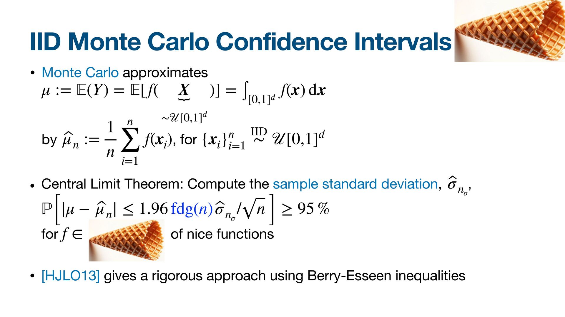
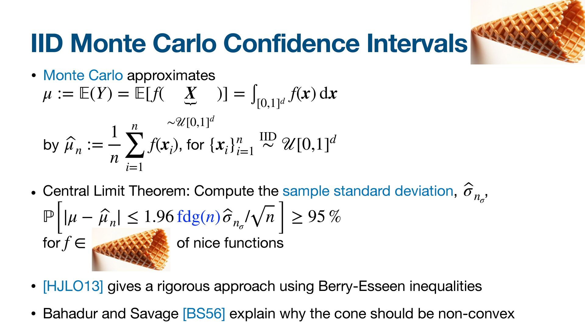
35. References [BS56] R. R. Bahadur and L. J. Savage, The nonexistence of certain statistical procedures in nonparametric problems, Ann. Math. Stat. 27 (1956), 1115–1122. [Gil15] M. B. Giles, Multilevel Monte Carlo methods, Acta Numer. 24 (2015), 259–328. [H00] F. J. Hickernell, What a ff ects the accuracy of quasi-Monte Carlo quadrature?, Monte Carlo and Quasi-Monte Carlo Methods 1998 (H. Niederreiter and J. Spanier, eds.), Springer-Verlag, Berlin, 2000, pp. 16–55. [HJLO13] F. J. Hickernell, L. Jiang, Y. Liu, and A. B. Owen, Guaranteed conservative fi xed width con fi dence intervals via Monte Carlo sampling, Monte Carlo and Quasi-{M}onte {C}arlo Methods 2012 (J. Dick, F. Y. Kuo, G. W. Peters, and I. H. Sloan, eds.), Springer Proceedings in Mathematics and Statistics, vol. 65, Springer-Verlag, Berlin, 2013, pp. 105–128. [HJ16] F. J. Hickernell and Ll. A. Jiménez Rugama, Reliable adaptive cubature using digital sequences, Monte Carlo and Quasi-Monte Carlo Methods: MCQMC, Leuven, Belgium, April 2014 (R. Cools and D. Nuyens, eds.), Springer Proceedings in Mathematics and Statistics, vol. 163, Springer-Verlag, Berlin, 2016, pp. 367–383.
36. References [HKS25] F. J. Hickernell, N. Kirk, and A. G. Sorokin, Quasi-Monte Carlo methods: What, why, and how?, submitted to MCQMC 2024 proceedings, https://doi.org/10.48550/arXiv.2502.03644, 2025+. [JH19] R. Jagadeeswaran and F. J. Hickernell, Fast automatic Bayesian cubature using lattice sampling, Stat. Comput. 29 (2019), 1215–1229. [JH22] R. Jagadeeswaran and F. J. Hickernell, Fast automatic Bayesian cubature using Sobol' sampling, Advances in Modeling and Simulation: Festschrift in Honour of Pierre L'Ecuyer (Z. Botev, A. Keller, C. Lemieux, and B. Tu ff i n, eds.), Springer, Cham, 2022, pp. 301–318. [JO25] A. Jain and A. B. Owen, Empirical Bernstein and betting con fi dence intervals for randomized quasi-Monte Carlo, in preparation to be submitted for publication, 2025+. [JH16] Ll. A. Jiménez Rugama and F. J. Hickernell, Adaptive multidimensional integration based on rank-1 lattices, Monte Carlo and Quasi-Monte Carlo Methods: MCQMC, Leuven, Belgium, April 2014 (R. Cools and D. Nuyens, eds.), Springer Proceedings in Mathematics and Statistics, vol. 163, Springer-Verlag, Berlin, 2016, pp. 407–422.
37. References [Kei96] B. D. Keister, Multidimensional quadrature algorithms, Computers in Physics 10 (1996), 119– 122. [LENOT24] P. L'Ecuyer, M. K. Nakayama, A. B. Owen, and B. Tu ffi n, Con fi dence intervals for randomized quasi-Monte Carlo estimators, WSC ’23: Proceedings of the Winter Simulation Conference, 2024, pp. 445–456. [MP09] A. Maurer and M. Pontil, Empirical Bernstein bounds and sample variance penalization, Proceedings of the 22nd Annual Conference on Learning Theory (COLT), 2009, pp. 1–9. [SJ24] A. G. Sorokin and R. Jagadeeswaran, On bounding and approximating functions of multiple expectations using quasi-Monte Carlo, Monte Carlo and Quasi-Monte Carlo Methods: MCQMC, Linz, Austria, July 2022 (A. Hinrichs, P. Kritzer, and F. Pillichshammer, eds.), Springer Proceedings in Mathematics and Statistics, Springer, Cham, 2024, pp. 583–589. [WSR24] I. Waubdy-Smith and A. Ramdas, Estimating means of bounded random variables by betting, J. Roy. Statist. Soc. B 86 (2024), 1–27.
38. Multilevel methods reduce computational cost [Gil15] μ := expectation 𝔼 [f( X ⏟ ∼ 𝒰 ([0,1]d) )] = integral ∫ [0,1]d f(x) dx ≈ sample mean 1 n n ∑ i=1 f(xi ) =: ̂ μn • The cost to evaluate is typically , so the cost to obtain is typically • If one can approximate by lower dimensional approximations, , then f(xi ) 𝒪 (d) |μ − ̂ μn | ≤ ε 𝒪 (dε−1−δ) f fs : [0,1]s → ℝ μ = 𝔼 [fs1 (X1:s1 )] μ(1) + 𝔼 [fs2 (X1:s2 ) − fs1 (X1:s1 )] μ(2) + ⋯ + 𝔼 [f(X1:d ) − fsL−1 (X1:sL−1 )] μ(L) • Balance the cost to approximate well and the total cost to obtain may be as small as as 𝒪 (nl sl ) μ(s) |μ − ̂ μn | ≤ ε 𝒪 (ε−1−δ) d, ε−1 → ∞