Dorfler__Benelux_2026.pdf

Transcript

1. Data-Enabled Predictive Control (DeePC) Florian D¨ orfler ETH Z¨ urich 45th Benelux Meeting on Systems and Control 1/31
2. Tribute: all Benelux topics today Fundamental Lemma [Willems, Rapisarda, & Markovsky ’05] subspace intersection methods [Moonen et al., ’89] PE in linear systems [Green & Moore, ’86] many recent variations & extensions [van Waarde et al., ’20] generalized low- rank version [Markovsky & Dörfler, ’20] deterministic data-driven control [Markovsky & Rapisarda, ’08] data-driven control of linear systems [de Persis & Tesi, ’19] regularizations & MPC scenario [Coulson et al., ’19] data informativity [van Waarde et al., ’20] LFT formulation [Berberich et al., ’20] … ? explicit implicit non-control applications: e.g., estimation. filtering, & SysID stabilization of nonlinear systems [de Persis & Tesi, ’21] robust stability & recursive feasibility [Berberich et al., ’20] (distributional) robustness [Coulson et al., ’20, Huang et al., ’21] regularizer from relaxed SysID [Dörfler et al., ’21] subspace predictive control [Favoreel et al., ’99] subspace methods [Breschi, Chiuso, & Formention ’22] instrumental variables [Wingerden et al., ’22] 1980s & earlier 2005-2008 today ARX methods [Chiuso et al., ’24] SysID via set membership [Witsenhausen & Schweppe, ’68] behavior meets subspace SysID they knew it all re-discovery & explosion of results 2019-2022 … … … nonlinear extensions: kernelization, lifting, LPV, … complex applications: robotics, power, health care … adaptive versions & linked with APD, PPO, … stochastic extensions: PCE, stoch. SPC/ID… no bottom up ? mainstream & canonical behavior & geometry: Grassmanian, convex/conic affine systems 2/31
3. Acknowledgements Jeremy Coulson Ivan Markovsky & Alberto Padoan + many many others Linbin Huang Andras Sasfi John Lygeros Alessandro Chiuso Roy Smith Keith Moffat 3/31
4. Thoughts on data in control systems increasing role of data-centric methods in science / engineering / industry due to • methodological advances in statistics, optimization, & machine learning (ML) • unprecedented availability of brute force: deluge of data & computational power • ...and frenzy surrounding big data & ML Make up your own opinion, but ML works too well to be ignored – also in control ?!? “ One of the major developments in control over the past decade – & one of the most important moving forward – is the interaction of ML & control systems. ” [CSS roadmap] !"#$%&''#($)#**+, !"#$%&'(()* !"#$%&'()&*+', & “clever solutions always lose vs. computationally scalable ones” −→ changes research culture 4/31
5. Scientific landscape long & rich history (auto-tuning, system identification, adaptive control, RL, ...) & vast & fragmented research landscape −→ useful direct / indirect classification ? x+ = f(x, u) y = h(x, u) y u direct data-driven control minimize control cost u, y subject to trajectory u, y compatible with data ud, yd model-based design system identification indirect (model-based) data-driven control minimize control cost u, y subject to trajectory u, y compatible with the model where model ∈ argmin fitting criterion ud, yd subject to model belongs to certain class 5/31
6. Indirect vs. direct • models are useful for design & beyond • modular → easy to debug & interpret • id = projection on model class • id = noise filtering • harder to propagate uncertainty through id • no (robust) separation principle → suboptimal • ... ? x+ = f(x, u) y = h(x, u) y u • some models are too complex to be useful • end-to-end → cheap & no experts needed • harder to inject side info but no bias error • noise handled in design • transparent: no unmodeled dynamics • possibly optimal but often less tractable • ... lots of pros, cons, counterexamples, & no universal conclusions [discussion] 6/31
7. Today’s menu 1. {behavioral systems} ∩ {subspace ID}: fundamental lemma 2. potent direct method: data-enabled predictive control DeePC 3. salient regularizations for robustification & inject side info 4. extensions to stochastic behaviors in the making 5. case studies: power system/electronics & building automation          my spiel on by now canonical topics blooming literature (∼3 ArXiv / week) for a few years already → tutorial [link] to get started • [link] to graduate school material • [link] to survey • [link] to related bachelor lecture • [link] to related publications DATA-DRIVEN CONTROL BASED ON BEHAVIORAL APPROACH: FROM THEORY TO APPLICATIONS IN POWER SYSTEMS Ivan Markovsky, Linbin Huang, and Florian Dörfler I. Markovsky is with ICREA, Pg. Lluis Companys 23, Barcelona, and CIMNE, Gran Capitàn, Barcelona, Spain (e-mail: imarkovsky@cimne.upc.edu), L. Huang and F. Dörfler are with the Automatic Control Laboratory, ETH Zürich, 8092 Zürich, Switzerland (e-mails: linhuang@ethz.ch, dorfler@ethz.ch). modeling). Modeling using observed data, possibly incorporating 7/31
8. the fundamental lemma
9. “The behavior is all there is.” Jan Willems’ behavioral system theory ...has been called useless & inaccessible ...yet we are all here still talking about it ! 8/31
10. Behavioral view on dynamical systems Definition: A discrete-time dynamical system is a 3-tuple (Z≥0 , W, B) where (i) Z≥0 is the discrete-time axis, (ii) W is the signal space, & (iii) B ⊆ WZ≥0 is the behavior.        B is the set of all trajectories Definition: The dynamical system (Z≥0 , W, B) is (i) linear if W is a vector space & B is a subspace of WZ≥0 (ii) time-invariant if wt ∈ B =⇒ wt+1 ∈ B (iii) admits input/output partition w = u, y with u free LTI system = shift-invariant subspace of trajectory space −→ abstract perspective suited for data-driven control “state space models are not a natural starting point for modelling [from data]” y u 9/31
11. Fundamental Lemma u(t) t u4 u2 u1 u3 u5 u6 u7 y(t) t y4 y2 y1 y3 y5 y6 y7 Given: data ud i yd i ∈ Rm+p & LTI complexity parameters lag ℓ order n set of all T-length trajectories = (u, y) ∈ R(m+p)T : ∃x ∈ RnT s.t. x+ = Ax + Bu , y = Cx + Du parametric state-space model raw data (every column is an experiment) colspan           ud 1,1 yd 1,1 ud 1,2 yd 1,2 ud 1,3 yd 1,3 ... ud 2,1 yd 2,1 ud 2,2 yd 2,2 ud 2,3 yd 2,3 ... . . . . . . . . . . . . ud T,1 yd T,1 ud T,2 yd T,2 ud T,3 yd T,3 ...           if and only if the trajectory matrix has rank m · T + n for all T ≥ ℓ 10/31
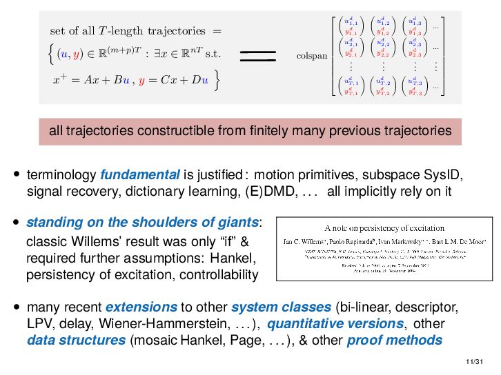
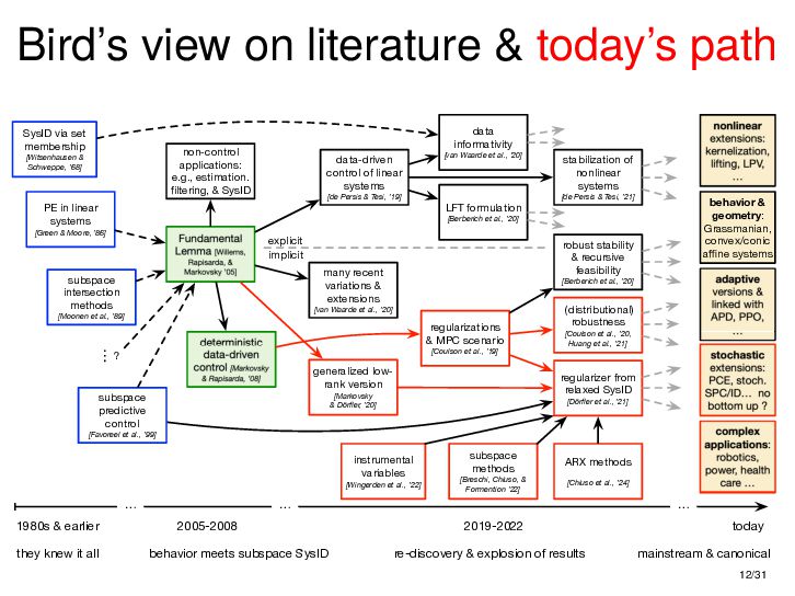
12. set of all T-length trajectories = (u, y) ∈ R(m+p)T : ∃x ∈ RnT s.t. x+ = Ax + Bu , y = Cx + Du parametric state-space model non-parametric model from raw data colspan           ud 1,1 yd 1,1 ud 1,2 yd 1,2 ud 1,3 yd 1,3 ... ud 2,1 yd 2,1 ud 2,2 yd 2,2 ud 2,3 yd 2,3 ... . . . . . . . . . . . . ud T,1 yd T,1 ud T,2 yd T,2 ud T,3 yd T,3 ...           all trajectories constructible from finitely many previous trajectories • terminology fundamental is justified : motion primitives, subspace SysID, signal recovery, dictionary learning, (E)DMD, ... all implicitly rely on it • standing on the shoulders of giants: classic Willems’ result was only “if” & required further assumptions: Hankel, persistency of excitation, controllability • many recent extensions to other system classes (bi-linear, descriptor, LPV, delay, Wiener-Hammerstein, ...), quantitative versions, other data structures (mosaic Hankel, Page, ...), & other proof methods 11/31
13. Bird’s view on literature & today’s path Fundamental Lemma [Willems, Rapisarda, & Markovsky ’05] subspace intersection methods [Moonen et al., ’89] PE in linear systems [Green & Moore, ’86] many recent variations & extensions [van Waarde et al., ’20] generalized low- rank version [Markovsky & Dörfler, ’20] deterministic data-driven control [Markovsky & Rapisarda, ’08] data-driven control of linear systems [de Persis & Tesi, ’19] regularizations & MPC scenario [Coulson et al., ’19] data informativity [van Waarde et al., ’20] LFT formulation [Berberich et al., ’20] … ? explicit implicit non-control applications: e.g., estimation. filtering, & SysID stabilization of nonlinear systems [de Persis & Tesi, ’21] robust stability & recursive feasibility [Berberich et al., ’20] (distributional) robustness [Coulson et al., ’20, Huang et al., ’21] regularizer from relaxed SysID [Dörfler et al., ’21] subspace predictive control [Favoreel et al., ’99] subspace methods [Breschi, Chiuso, & Formention ’22] instrumental variables [Wingerden et al., ’22] 1980s & earlier 2005-2008 today ARX methods [Chiuso et al., ’24] SysID via set membership [Witsenhausen & Schweppe, ’68] behavior meets subspace SysID they knew it all re-discovery & explosion of results 2019-2022 … … … nonlinear extensions: kernelization, lifting, LPV, … complex applications: robotics, power, health care … adaptive versions & linked with APD, PPO, … stochastic extensions: PCE, stoch. SPC/ID… no bottom up ? mainstream & canonical behavior & geometry: Grassmanian, convex/conic affine systems 12/31
14. A Benelux topic throughout time Fundamental Lemma [Willems, Rapisarda, & Markovsky ’05] subspace intersection methods [Moonen et al., ’89] PE in linear systems [Green & Moore, ’86] many recent variations & extensions [van Waarde et al., ’20] generalized low- rank version [Markovsky & Dörfler, ’20] deterministic data-driven control [Markovsky & Rapisarda, ’08] data-driven control of linear systems [de Persis & Tesi, ’19] regularizations & MPC scenario [Coulson et al., ’19] data informativity [van Waarde et al., ’20] LFT formulation [Berberich et al., ’20] … ? explicit implicit non-control applications: e.g., estimation. filtering, & SysID stabilization of nonlinear systems [de Persis & Tesi, ’21] robust stability & recursive feasibility [Berberich et al., ’20] (distributional) robustness [Coulson et al., ’20, Huang et al., ’21] regularizer from relaxed SysID [Dörfler et al., ’21] subspace predictive control [Favoreel et al., ’99] subspace methods [Breschi, Chiuso, & Formention ’22] instrumental variables [Wingerden et al., ’22] 1980s & earlier 2005-2008 today ARX methods [Chiuso et al., ’24] SysID via set membership [Witsenhausen & Schweppe, ’68] behavior meets subspace SysID they knew it all re-discovery & explosion of results 2019-2022 … … … nonlinear extensions: kernelization, lifting, LPV, … complex applications: robotics, power, health care … adaptive versions & linked with APD, PPO, … stochastic extensions: PCE, stoch. SPC/ID… no bottom up ? mainstream & canonical behavior & geometry: Grassmanian, convex/conic affine systems 13/31
15. Data-enabled Predictive Control (DeePC)
16. Output Model Predictive Control (MPC) minimize u, x, y Tfuture k=1 ∥yk − rk ∥2 Q + ∥uk ∥2 R subject to xk+1 = Axk + Buk yk = Cxk + Duk ∀k ∈ {1, . . . , Tfuture } xk+1 = Axk + Buk yk = Cxk + Duk ∀k ∈ {−Tini − 1, . . . , 0} uk ∈ U yk ∈ Y ∀k ∈ {1, . . . , Tfuture } quadratic cost with R ≻ 0, Q ⪰ 0 & ref. r model for prediction with k ∈ [1, Tfuture ] model for estimation with k ∈ [−Tini − 1, 0] & Tini ≥ lag (many flavors) hard operational or safety constraints “[MPC] has perhaps too little system theory and too much brute force [...], but MPC is an area where all aspects of the field [...] are in synergy.” – Willems ’07 Elegance aside, for an LTI plant, deterministic, & with known model, MPC is the gold standard of control. 14/31
17. Data-enabled Predictive Control (DeePC) minimize g, u, y Tfuture k=1 ∥yk − rk ∥2 Q + ∥uk ∥2 R subject to H ud yd · g =     uini yini u y     uk ∈ U yk ∈ Y ∀k ∈ {1, . . . , Tfuture } quadratic cost with R ≻ 0, Q ⪰ 0 & ref. r non-parametric representation for prediction & estimation hard operational or safety constraints • real-time measurements (uini , yini ) for estimation • trajectory matrix H ud yd from past experimental data updated online collected offline (could be adapted online) → equivalent to MPC in deterministic LTI case ... but needs to be robustified in case of noise / nonlinearity ! 15/31
18. Regularizations make it work minimize g, u, y, σ Tfuture k=1 ∥yk − rk ∥2 Q + ∥uk ∥2 R + λy ∥σ∥p + λg h(g) subject to H ud yd · g =     uini yini u y     +     0 σ 0 0     uk ∈ U yk ∈ Y ∀k ∈ {1, . . . , Tfuture } measurement noise → infeasible yini estimate → estimation slack σ → moving-horizon least-square filter noisy or nonlinear (offline) data matrix → any (u y ) feasible → add regularizer h(g) Bayesian intuition: regularization ⇔ prior, e.g., h(g) = ∥g∥1 sparsely selects {trajectory matrix columns} ∼ low-order basis ∼ low-rank surrogate Robustness intuition: regularization ⇔ robustifies, e.g., in a simple case min x max ∥∆∥≤ρ ∥(A+∆)x−b∥ ≤ tight min x max ∥∆∥≤ρ ∥Ax−b∥+∥∆x∥ = min x ∥Ax−b∥+ρ∥x∥ 16/31
19. it’s simple & it works
20. Works very well across case studies ...especially when first-principle models are hard or impossible to get 17/31
21. regularization ⇕ incorporating priors + implicit SysID
22. Regularization = relaxing low-rank approximation in pre-processing minimizeu,y,g control cost u, y subject to u y = H ˆ u ˆ y g where ˆ u ˆ y ∈ argmin ˆ u ˆ y − ud yd subject to rank H ˆ u ˆ y = mL + n ↓ sequence of convex relaxations ↓ minimizeu,y,g control cost u, y + λg · g 1 subject to u y = H ud yd g ℓ1 -regularization = surrogate for low-rank approximation & smoothened order selection    optimal control    low-rank approximation !"#$%&'"##()*#$+ realized closed-loop cost λg 18/31
23. Regularization ⇔ reformulate subspace ID partition data as in subspace ID: H ud yd ∼     Up Yp Uf Yf     (m + p)Tini (m + p)Tfuture ID of optimal multi-step predictor as in SPC : K⋆ = YF Up Yp Uf †    → indirect SysID + control problem minimize u,y control cost(u, y) subject to y = K⋆   uini yini u   where K⋆ = argmin K YF − K   Up Yp Uf   The above is equivalent to regularized DeePC where Proj ud yd projects orthogonal to ker Up Yp Uf minimize g,u,y control cost(u, y) + λg Proj ud yd g p subject to H ud yd · g =     uini yini u y     19/31
24. Regularizations applied to stochastic LTI system & hyper-parameter selection g p Proj ud yd g p Hanke-Raus heuristic (often) reveals 20/31
25. time for a case study
26. Case study: wind turbine • turbine & grid model unknown to commissioning engineer & operator • detailed industrial model: 37 states & highly nonlinear (abc ↔ dq, MPTT, PLL, power specs, dynamics, etc.) • weak grid → oscillations + sync loss • disturbance to be rejected by DeePC !"#" $%&&'$#(%) *(#+%,#-"!!(#(%)"&-$%)#.%& %/$(&&"#(%) %0/'.1'! h(g) = g 2 2 h(g) = g 1 h(g) = Proj ud yd g 2 2 2''34-"$#(1"#'! 2''34-"$#(1"#'! regularizer tuning h(g) = g 2 2 h(g) = g 1 h(g) = Proj ud yd g 2 2 Hanke-Raus heuristic 21/31
27. Case study +++ : wind farm SG 1 SG 2 SG 3 1 2 3 4 5 6 7 9 8 IEEE nine-bus system wind farm 1 2 3 4 5 6 7 8 9 10 • high-fidelity models for turbines, machines, & IEEE-9-bus system • fast frequency response via decentralized DeePC at turbines h(g) = Proj ud yd g 2 2 subspace ID + control 22/31
28. Pragmatic view on nonlinear systems na¨ ıve insight : every system is bi-/linear in large/∞-dimensions → Carleman, Volterra, Fliess, Koopman, Sturm-Liouville methods → nonlinear dynamics can be approximated by LTI on finite horizon regularization singles out relevant features / basis functions in data test on 100kW grid-connected inverter → going in vivo soon 80% of total operation range works spectacularly & reliably → why ? 23/31
29. regularization ⇕ robustification
30. Distributional robustification beyond LTI • problem abstraction : minx∈X c ξ, x = minx∈X Eξ∼P c (ξ, x) where ξ denotes measured data from the empirical distribution P = δ ξ ⇒ poor out-of-sample performance of above sample-average solution x⋆ for real problem: Eξ∼P c (ξ, x⋆) where P is the unknown distribution of ξ • distributionally robust formulation accounting for all (possibly nonlinear) stochastic processes that could have generated the data inf x∈X sup Q∈Bϵ (P) Eξ∼Q c (ξ, x) where Bϵ (P) is an ϵ-Wasserstein ball Bϵ (P) = P : inf Π ξ − ξ p dΠ ≤ ϵ theorem: inf sup · · · = DeePC + ∥g∥⋆ p -regularizer ˆ ξ ξ ˆ P P Π 24/31
31. SysID ≫ ? ≪ DeePC
32. Comparison: direct vs. indirect control indirect ID-based data-driven control minimize control cost u, y subject to u, y satisfy parametric model where model ∈ argmin id cost ud, yd subject to model ∈ LTI(n, ℓ) class ID ID projects data on LTI class to learn predictor • removes noise & thus lowers variance error • suffers bias error if plant is not in LTI(n, ℓ) • no uncertainty prop. direct regularized data-driven control minimize control cost u, y + λ· regularizer subject to u, y consistent with ud, yd data • no de-noising & no bias • regularization robustifies prediction (not predictor) • trade-off ID & control costs take-away : ID wins if model class is known, noise is well behaved, & control doesn’t bias ID. Else regularized DeePC beats ID [proofs by Padova teams]. 25/31
33. towards a stochastic behavioral systems theory
34. Getting the definition right & simple inputs & outputs linearity/ subspace property time-invariance, low order, causality, … multi-step predictor recursive model … … models: ARX, state space… impulse response matrix + Gaussianity “The behavior is all there is.” Gaussian behavior: trajectories are distributed as a Gaussian process     uini yini u y     ∼ N(µw , Σw ) Identification of (µw , Σw ) from sample correlation Prediction: y|uini , yini , u ∼ N  M   uini yini u   , Σ   obtained by closed-form conditioning y on uini , yini , u Conditioning 26/31
35. Old friends & new perspectives Predictive distribution y|uini , yini , u ∼ N  M   uini yini u   , Σ   with (M, Σ) =(ˆ µ,ˆ Σ) estimated → M = YF Up Yp Uf † subspace predictor & Σ = 1 # data Yf Proj ud yd previous regularizer Y ⊤ f Certainty-equivalence control: minu E N(ˆ µ,ˆ Σ) [cost(u, y)] = SPC Distributional uncertainty: real (µ, Σ) differ from (ˆ µ, ˆ Σ) −→ optimism    min u min µ EN(µ,Σ) [cost(u, y)] s.t. DKL N(µ, Σ) N(ˆ µ, ˆ Σ) ≤ ϵ = regularized DeePC −→ robust    min u max µ EN(µ,Σ) [cost(u, y)] s.t. DKL N(µ, Σ) N(ˆ µ, ˆ Σ) ≤ ϵ ⇒ new convex formulation 27/31
36. Leveraging the predictor’s variance time y et et+1 . . . Predicted Realized   et et+1 . . .   ∼ N(0, Σ) → et , et+1 , . . . correlated! −→ variance shaping by feedbacking error u = uff + Kcausal e −→ predictive distribution y = Mini Mu   uini yini uff   mean ˆ µ + (Mu Kcausal + I) e controlled variance min uff ,Kcausal E[cost(u, y)] = cost(uff , ˆ µ) + tr R · Σu Kcausal ΣK⊤ causal + tr Q · (Mu Kcausal + I)Σ(Mu Kcausal + I)⊤ Σy = mean cost + LQG variance cost 28/31
37. Building control benchmark [Gwerder & T¨ odtli, Siemens, ’05] • model: 7th order, LTI, thermal RC circuit • inputs: heating & cooling • disturbances: outside air temperature, solar radiation, & occupancy • constraints: [21◦, 26◦] room temperature to be met with 99% probability • disturbance forecast available with temporally increasing uncertainty 0 s outside envelope. The window and free cooling system heat transfer coefficients are chang with blind position u3 and free cooling activity u4 , respectively. To represent the dynamic behavior of a real building, thermal capacities are assigned to the lumped thermal room kn (Cr ), the outside envelope (Co1 , Co2 , Co3 ) and the inner parts of the building (Ci1 , Ci2 , Ci3 ). T modeled windows have no thermal capacity. The building model can be written in a pseud linear state space representation (3), where the state vector x is given by (4), the disturbanc input vector v by (5) and the state space matrices by (6)-(9). Figure 1. Schematic diagram of the building model ( ) [ ] ) ( ) ( ) ( )) ( ), ( ( ) ( ) ( ) ( ) ( ) ( ) ( ) ( * 4 1 , , t x C t y t u t v t x B t u t x B t v B t v B t u B t x A t x u i i i xu i vu v u = + + + + = ∑ = 4 4 4 4 4 3 4 4 4 4 4 2 1 & [ ] ) ( ) ( ) ( ) ( ) ( ) ( ) ( ) ( 3 2 1 3 2 1 t t t t t t t t x o o o i i i r T ϑ ϑ ϑ ϑ ϑ ϑ ϑ = [ ] ) ( ) ( ) ( ) ( ) ( ) ( 1 0 t q t q t q t t t v i s s oawb oa T & & & ϑ ϑ = ⎥ ⎥ ⎥ ⎥ ⎤ ⎢ ⎢ ⎢ ⎢ ⎡ + − + + + + − 1 2 1 2 1 1 1 1 4 1 4 1 1 0 0 0 0 0 0 0 0 i i i i i i i r o r i r i r i o i w a a C K C K K C K C K C K C K C K K K K C n & context: SysID is often the economic barrier to automating old buildings → data gathering inputs, outputs, outside temp., & weather forecast → Gaussian behavior with outside temp. input (uncertain forecast) 29/31
38. Some open-loop sample trajectories without covariance feedback with covariance feedback −→ covariance feedback significantly reduces variance & lowers heating control effort at same level of constraint satisfaction −→ receding-horizon control over 2 days reduces heating by 31% 30/31
39. Conclusions take-away: simple, working, & certified method • matrix time series as predictive model • robustness & side-info by regularization • Gaussian behaviors for stochastic systems no-free-lunch ? downside to models ? • no sparsity & more compute ↮ bitter lesson ongoing work • complex system classes & adaptation • applications with a true “business case” SG 1 SG 2 SG 3 1 2 3 4 5 6 7 9 8 IEEE nine-bus system wind farm 1 2 3 4 5 6 7 8 9 10 nothing was new today other than the perspective 31/31
40. Thanks !