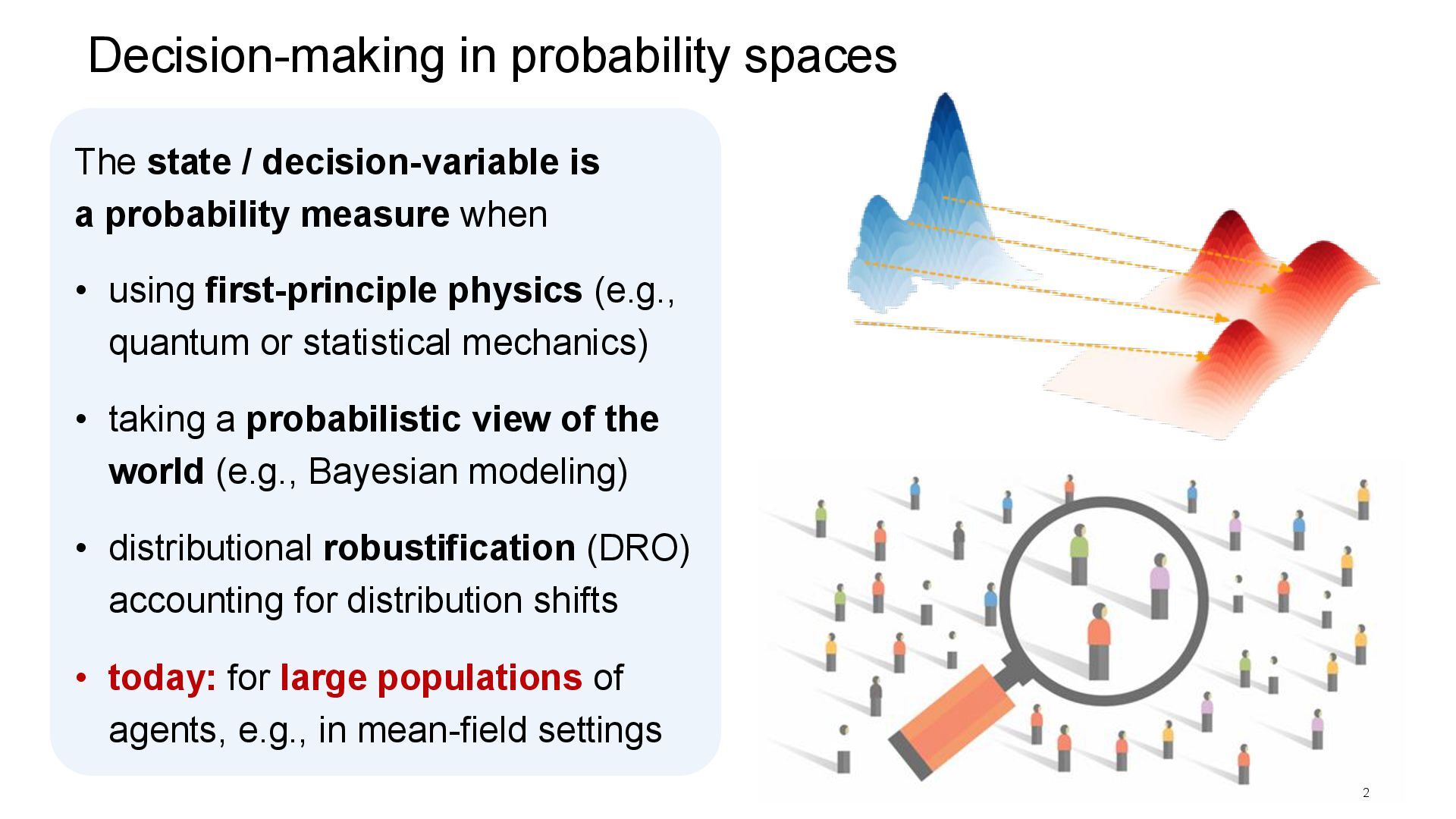
probability measure when • using first-principle physics (e.g., quantum or statistical mechanics) • taking a probabilistic view of the world (e.g., Bayesian modeling) • distributional robustification (DRO) accounting for distribution shifts • today: for large populations of agents, e.g., in mean-field settings 2
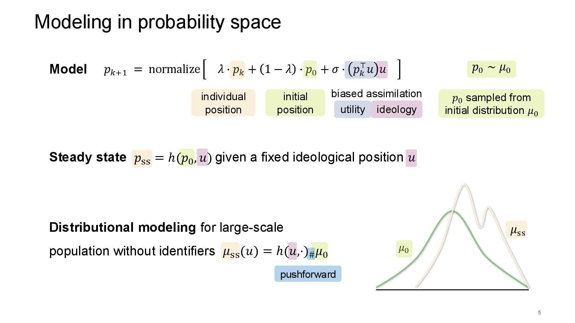
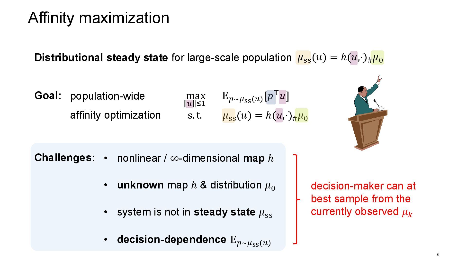
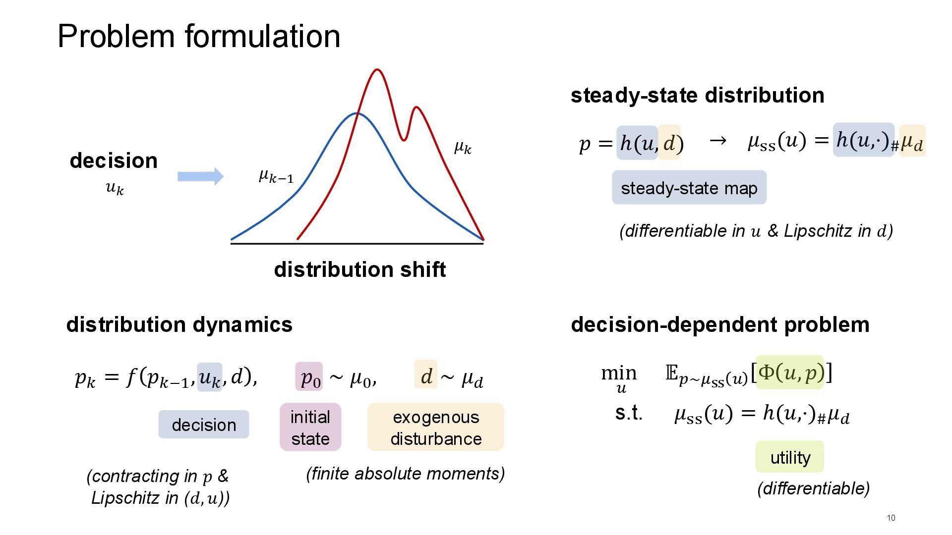
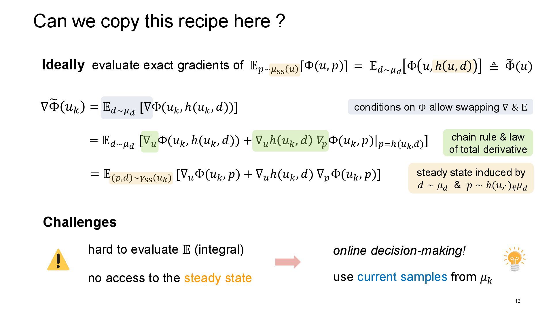
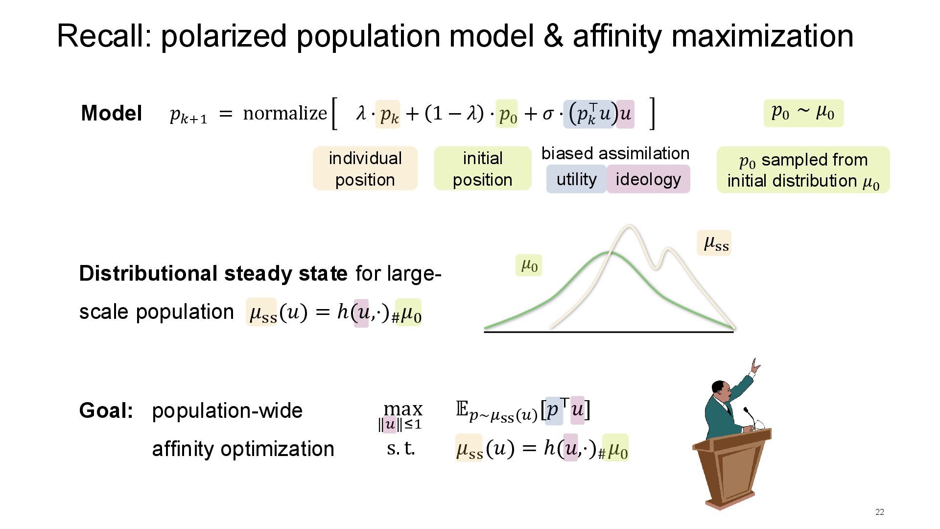
[𝑝⊤𝑢] Affinity maximization 6 Goal: population-wide affinity optimization Distributional steady state for large-scale population Challenges: • nonlinear / ∞-dimensional map ℎ • unknown map ℎ & distribution 𝜇0 • system is not in steady state 𝜇ss • decision-dependence 𝔼𝑝∼𝜇ss(𝑢) decision-maker can at best sample from the currently observed 𝜇𝑘 𝜇ss (𝑢) = ℎ(𝑢,⋅)# 𝜇0
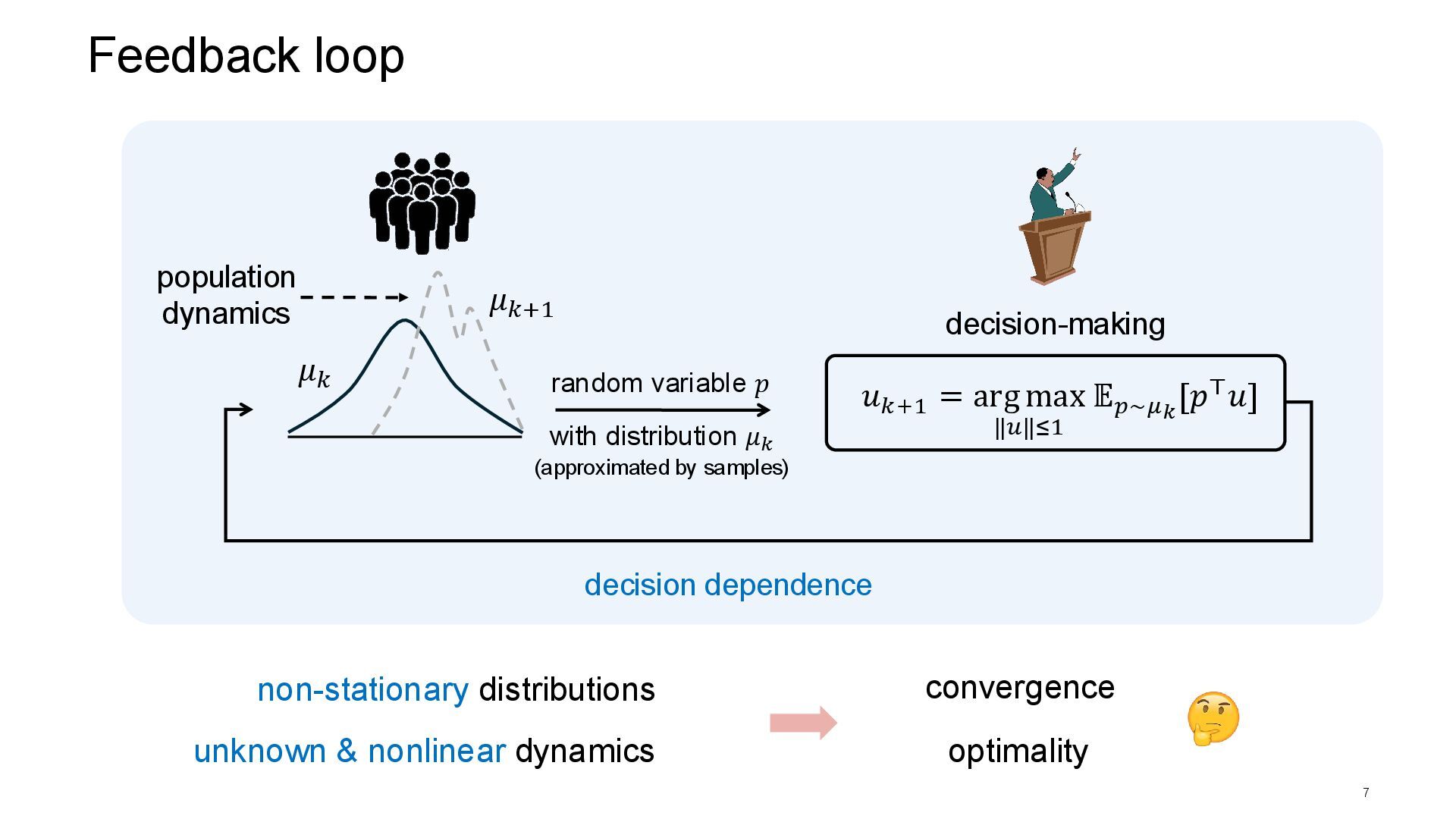
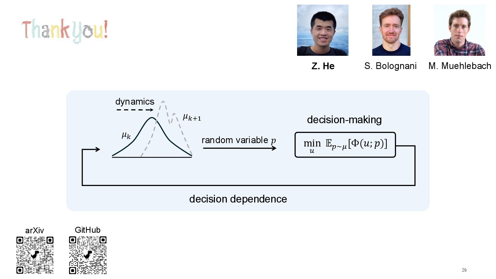
optimality random variable 𝑝 decision-making 𝜇𝑘 decision dependence population dynamics 𝜇𝑘+1 with distribution 𝜇𝑘 (approximated by samples) 𝑢𝑘+1 = arg max ‖𝑢‖≤1 𝔼𝑝∼𝜇𝑘 [𝑝⊤𝑢]
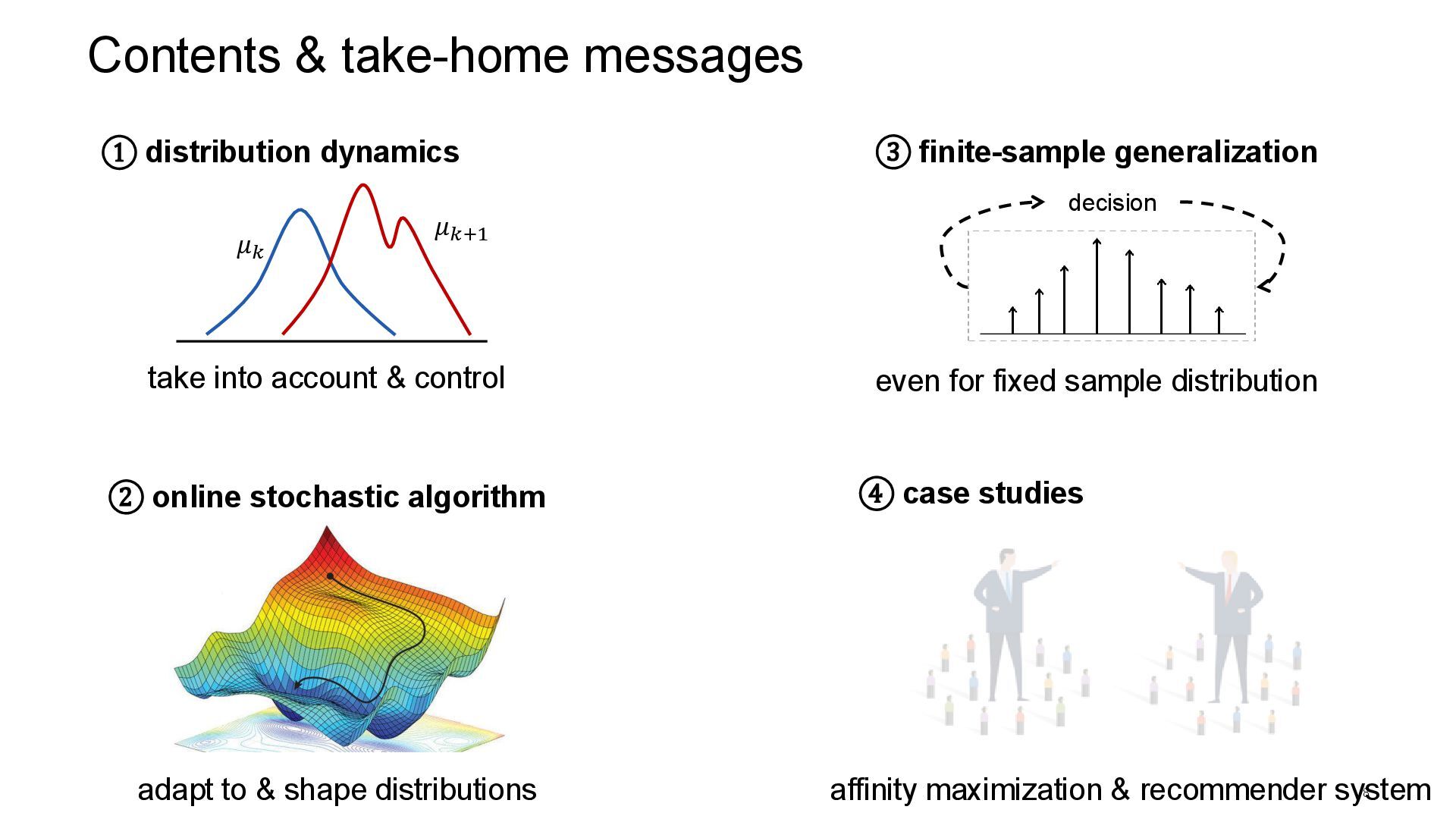
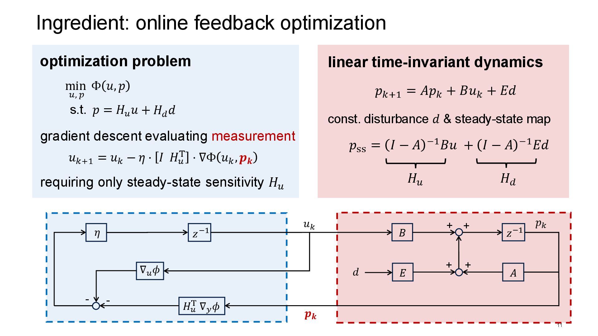
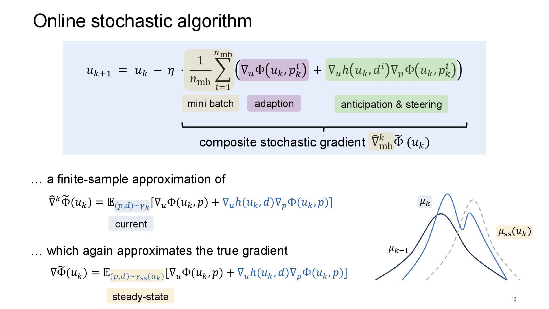
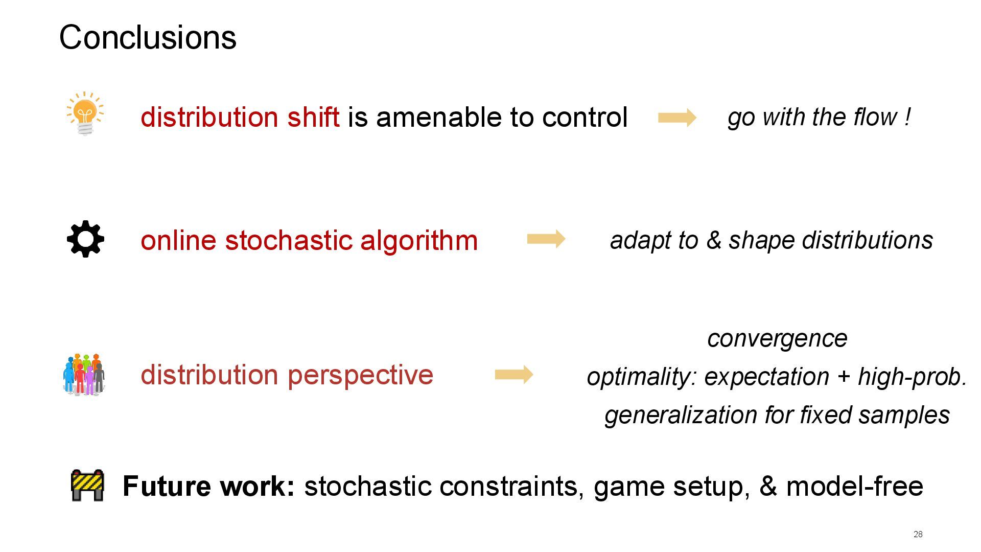
generalization ② online stochastic algorithm decision take into account & control even for fixed sample distribution adapt to & shape distributions 𝜇𝑘 𝜇𝑘+1 ④ case studies affinity maximization & recommender system
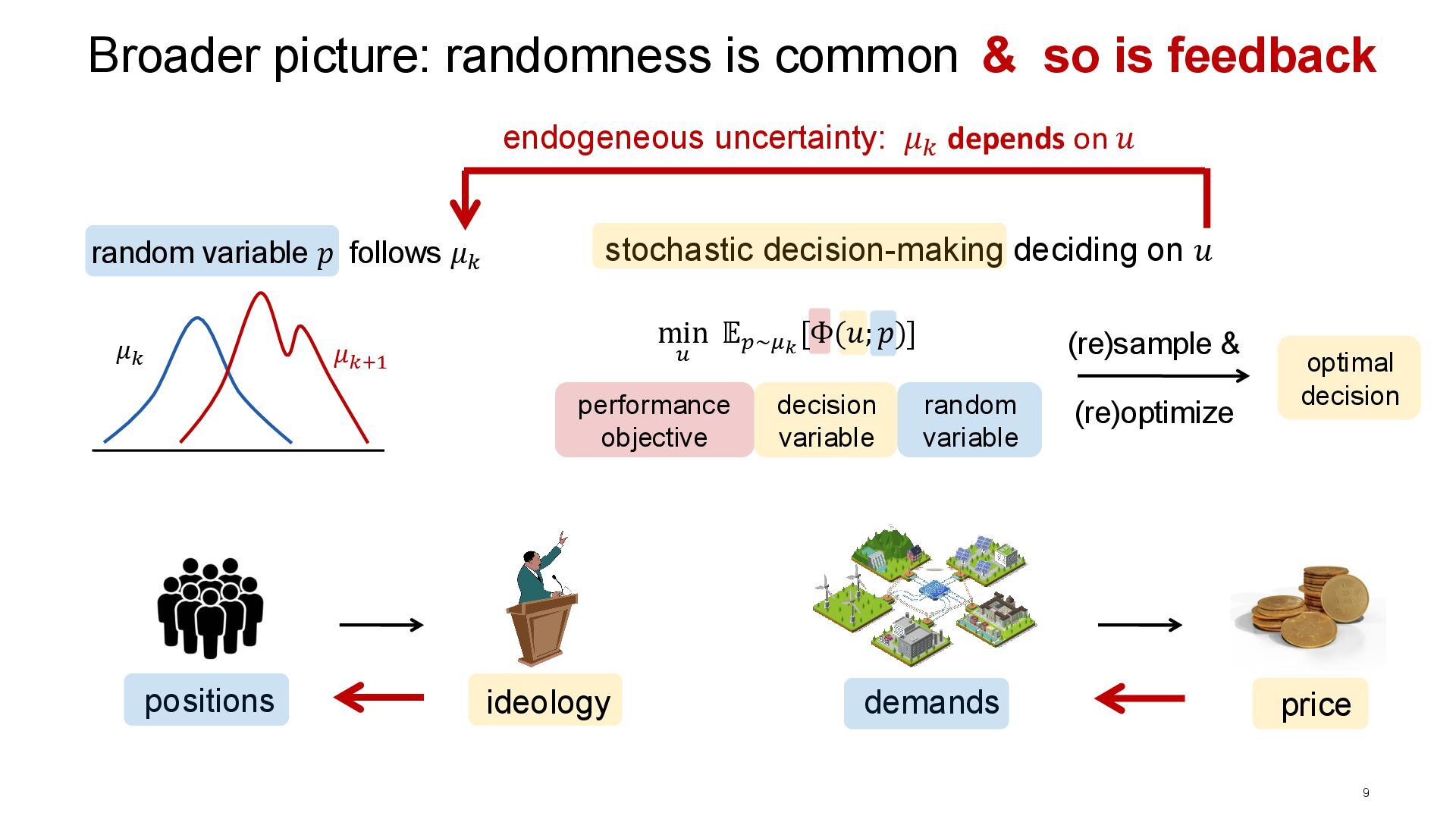
picture: randomness is common (re)sample & random variable 𝑝 follows 𝜇𝑘 decision variable random variable performance objective positions ideology demands price optimal decision & so is feedback endogeneous uncertainty: 𝜇𝑘 depends on 𝑢 min 𝑢 𝔼𝑝∼𝜇𝑘 [Φ(𝑢; 𝑝)]
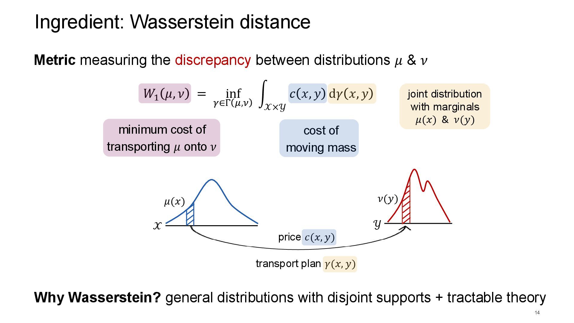
𝑥, 𝑦 d𝛾 𝑥, 𝑦 Ingredient: Wasserstein distance 14 𝜇(𝑥) Metric measuring the discrepancy between distributions 𝜇 & 𝜈 cost of moving mass 𝜈(𝑦) transport plan 𝛾(𝑥, 𝑦) minimum cost of transporting 𝜇 onto 𝜈 Why Wasserstein? general distributions with disjoint supports + tractable theory price 𝑐(𝑥, 𝑦) joint distribution with marginals 𝜇(𝑥) & 𝜈(𝑦) 𝒳 𝒴
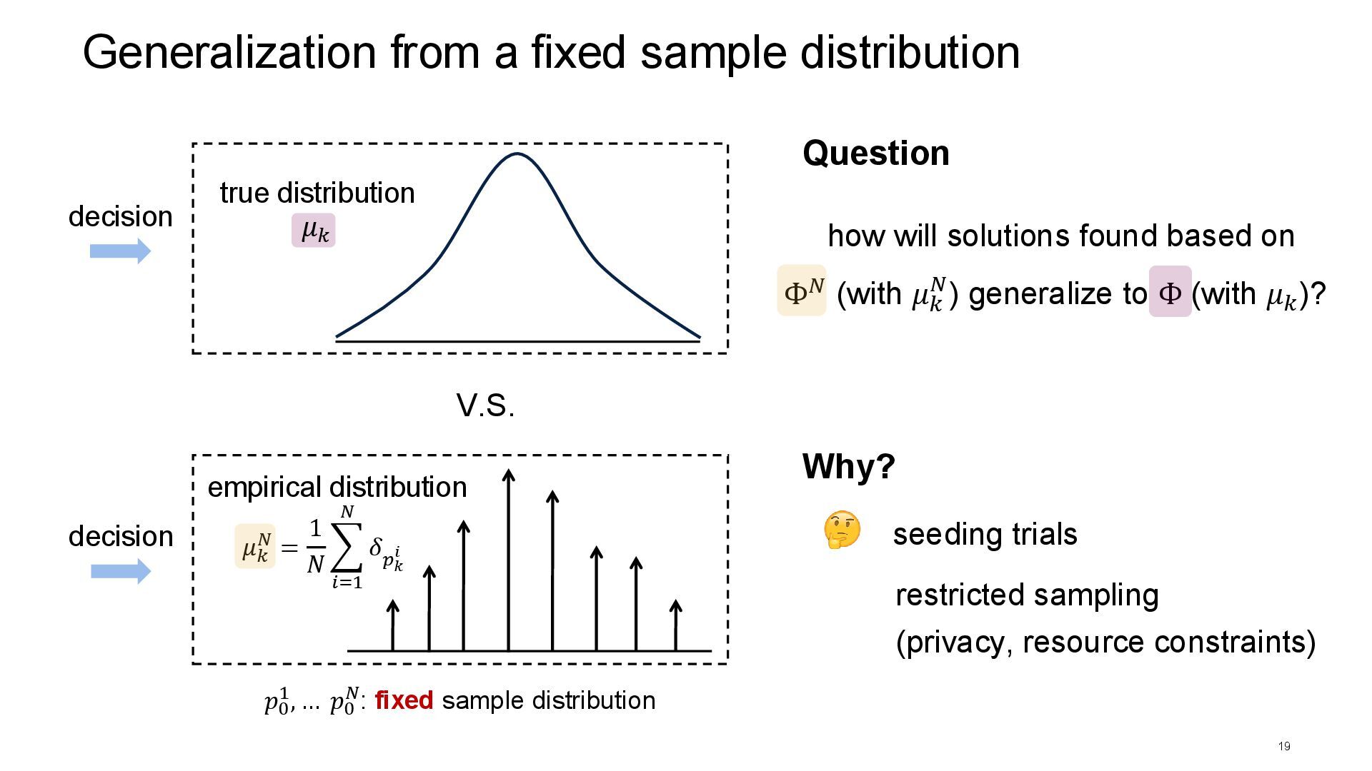
how will solutions found based on Generalization from a fixed sample distribution 19 true distribution empirical distribution Why? seeding trials restricted sampling (privacy, resource constraints) decision decision Question V.S. 𝜇𝑘 𝜇𝑘 𝑁 = 1 𝑁 𝑖=1 𝑁 𝛿 𝑝𝑘 𝑖 𝑝0 1, … 𝑝0 𝑁: fixed sample distribution
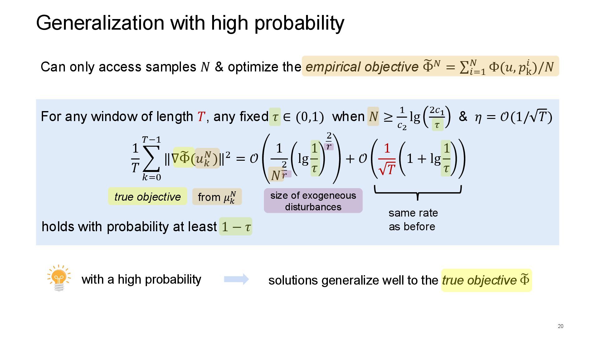
& optimize the empirical objective ෩ Φ𝑁 = σ 𝑖=1 𝑁 Φ(𝑢, 𝑝k 𝑖 )/𝑁 with a high probability solutions generalize well to the true objective ෩ Φ For any window of length 𝑇, any fixed 𝜏 ∈ (0,1) when 𝑁 ≥ 1 𝑐2 lg 2𝑐1 𝜏 & 𝜂 = 𝒪(1/ 𝑇) holds with probability at least 1 − 𝜏 size of exogeneous disturbances from 𝜇𝑘 𝑁 1 𝑇 𝑘=0 𝑇−1 ‖∇෩ Φ(𝑢𝑘 𝑁)‖2 = 𝒪 1 𝑁 2 𝑟 lg 1 𝜏 2 𝑟 + 𝒪 1 𝑇 1 + lg 1 𝜏 true objective same rate as before
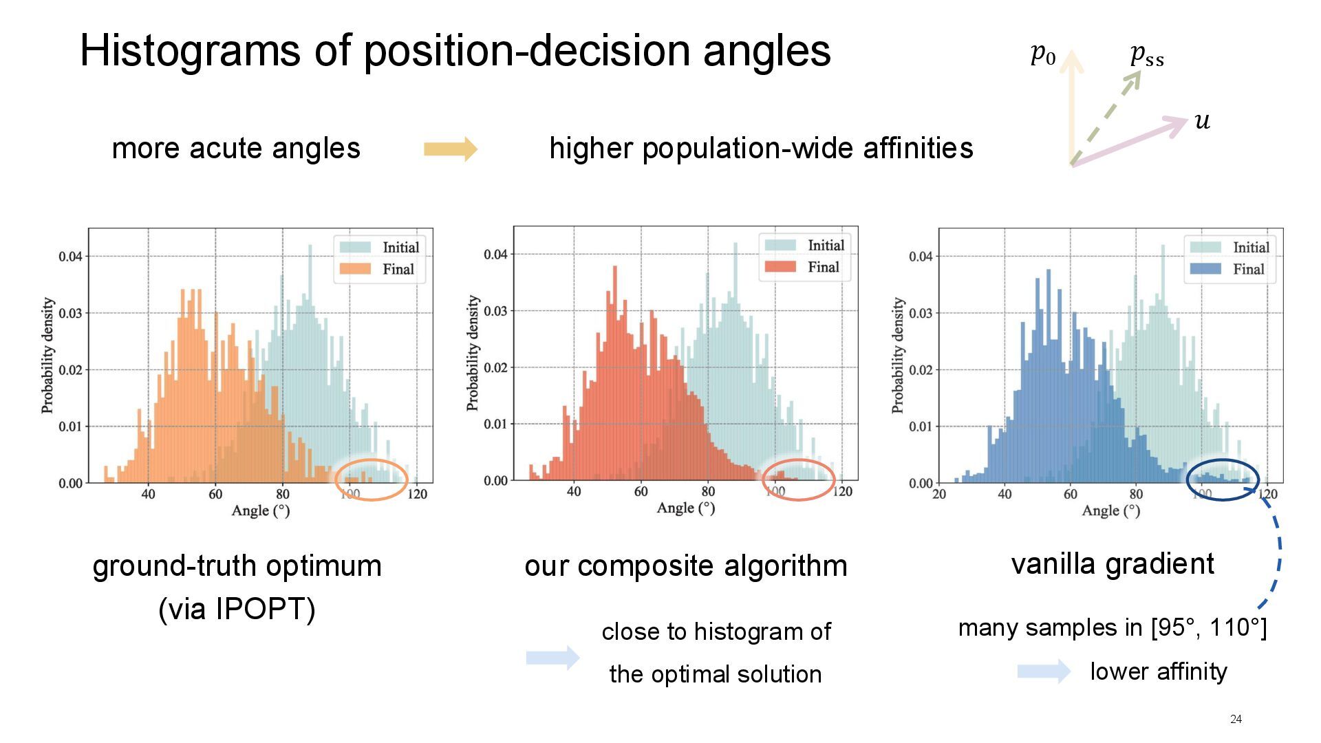
gradient our composite algorithm higher population-wide affinities more acute angles close to histogram of the optimal solution many samples in [95°, 110°] lower affinity 𝑢 𝑝0 𝑝ss
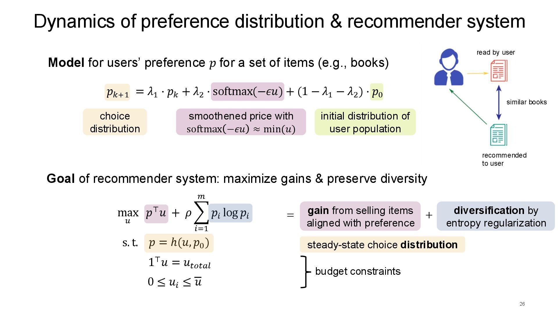
smoothened price with softmax −𝜖𝑢 ≈ min(𝑢) Model for users’ preference 𝑝 for a set of items (e.g., books) initial distribution of user population Goal of recommender system: maximize gains & preserve diversity gain from selling items aligned with preference diversification by entropy regularization 𝑝𝑘+1 = 𝜆1 ⋅ 𝑝𝑘 + 𝜆2 ⋅ softmax(−𝜖𝑢) + (1 − 𝜆1 − 𝜆2 ) ⋅ 𝑝0 max 𝑢 𝑝⊤𝑢 + 𝜌 𝑖=1 𝑚 𝑝𝑖 log 𝑝𝑖 𝑝 = ℎ(𝑢, 𝑝0 ) 0 ≤ 𝑢𝑖 ≤ 𝑢 s. t. 1⊤𝑢 = 𝑢𝑡𝑜𝑡𝑎𝑙 = + steady-state choice distribution budget constraints read by user recommended to user similar books
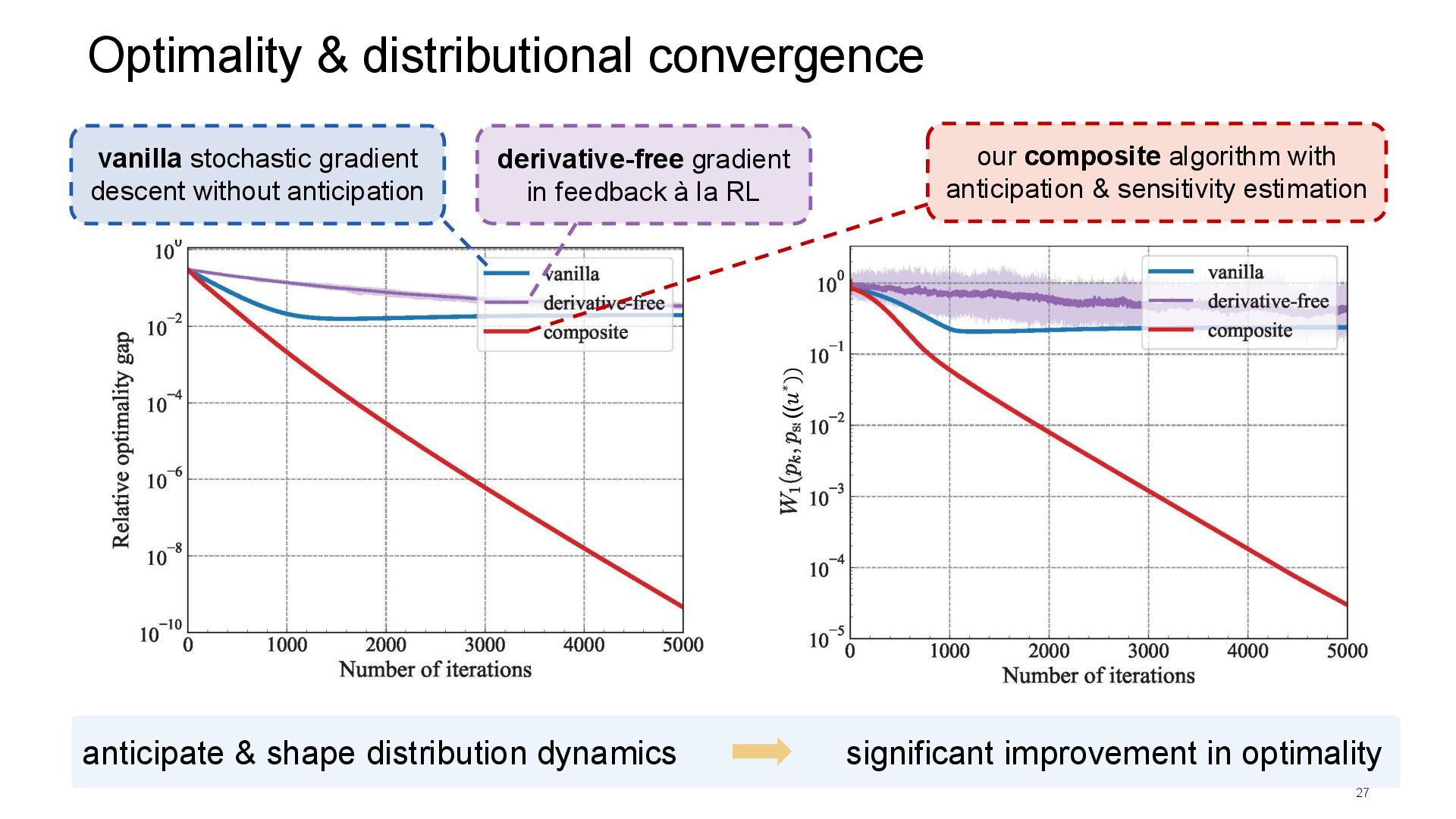
dynamics significant improvement in optimality vanilla stochastic gradient descent without anticipation our composite algorithm with anticipation & sensitivity estimation derivative-free gradient in feedback à la RL