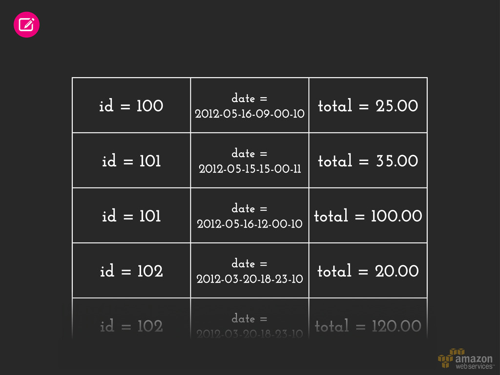
= 101 date = 2012-05-15-15-00-11 total = 35.00 id = 101 date = 2012-05-16-12-00-10 total = 100.00 id = 102 date = 2012-03-20-18-23-10 total = 20.00 id = 102 date = 2012-03-20-18-23-10 total = 120.00
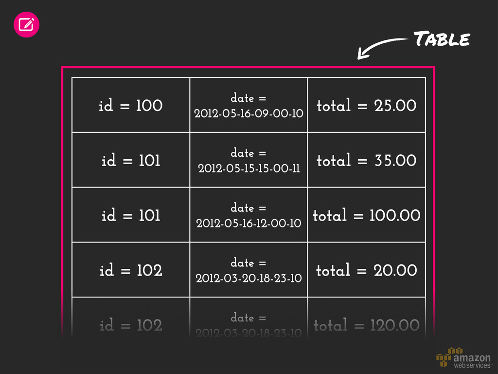
= 101 date = 2012-05-15-15-00-11 total = 35.00 id = 101 date = 2012-05-16-12-00-10 total = 100.00 id = 102 date = 2012-03-20-18-23-10 total = 20.00 id = 102 date = 2012-03-20-18-23-10 total = 120.00 Table
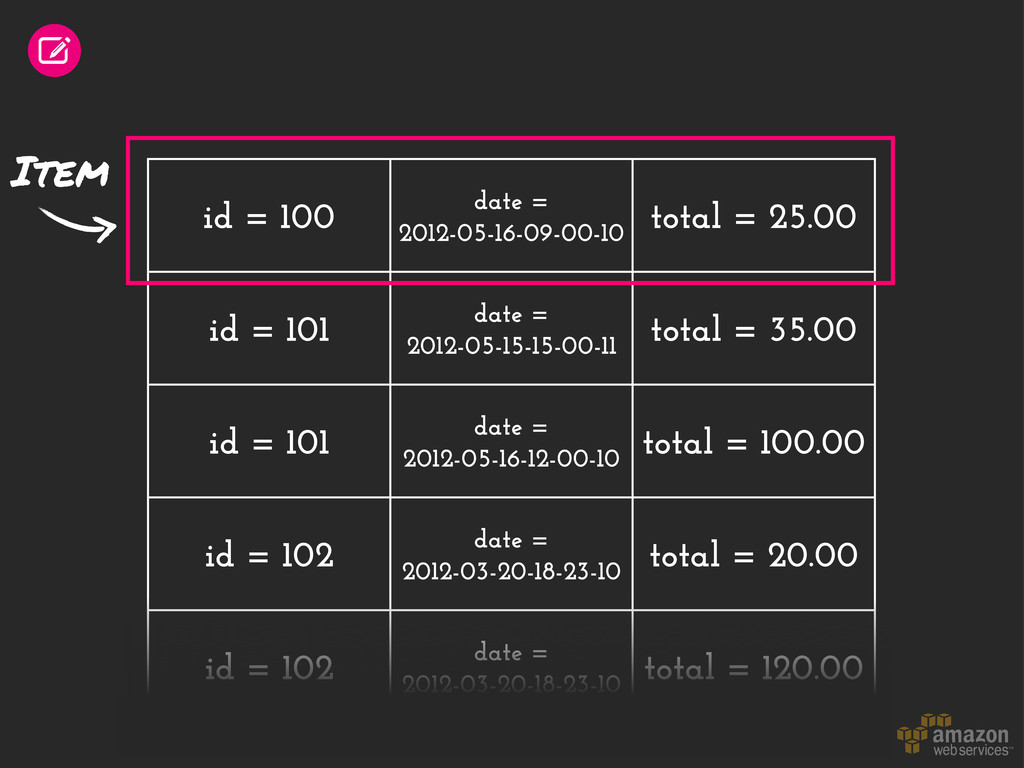
= 101 date = 2012-05-15-15-00-11 total = 35.00 id = 101 date = 2012-05-16-12-00-10 total = 100.00 id = 102 date = 2012-03-20-18-23-10 total = 20.00 id = 102 date = 2012-03-20-18-23-10 total = 120.00 Item
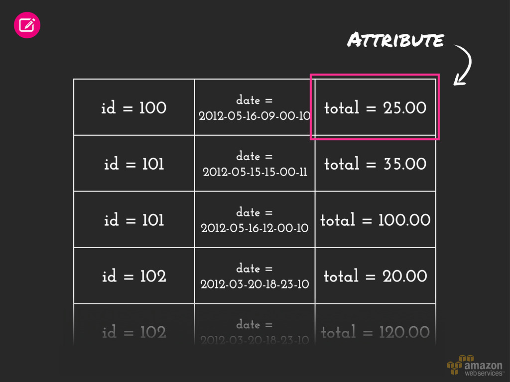
= 101 date = 2012-05-15-15-00-11 total = 35.00 id = 101 date = 2012-05-16-12-00-10 total = 100.00 id = 102 date = 2012-03-20-18-23-10 total = 20.00 id = 102 date = 2012-03-20-18-23-10 total = 120.00 Attribute
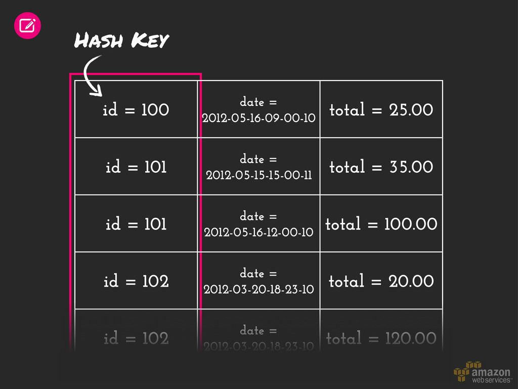
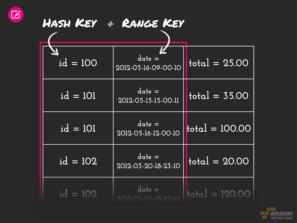
= 101 date = 2012-05-15-15-00-11 total = 35.00 id = 101 date = 2012-05-16-12-00-10 total = 100.00 id = 102 date = 2012-03-20-18-23-10 total = 20.00 id = 102 date = 2012-03-20-18-23-10 total = 120.00 Hash Key
= 101 date = 2012-05-15-15-00-11 total = 35.00 id = 101 date = 2012-05-16-12-00-10 total = 100.00 id = 102 date = 2012-03-20-18-23-10 total = 20.00 id = 102 date = 2012-03-20-18-23-10 total = 120.00 Hash Key Range Key +
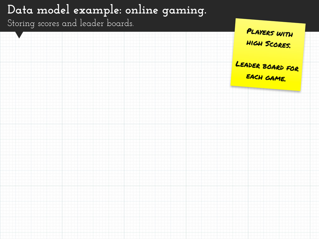
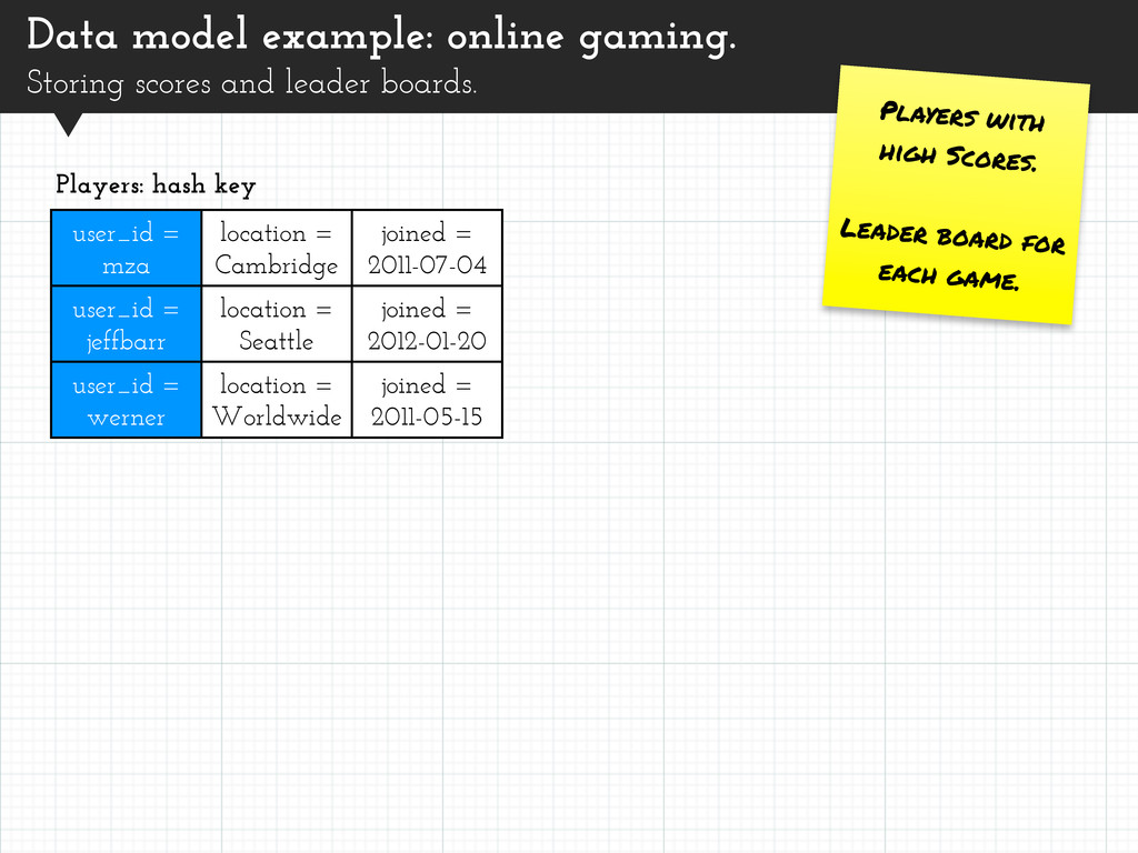
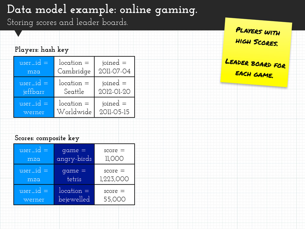
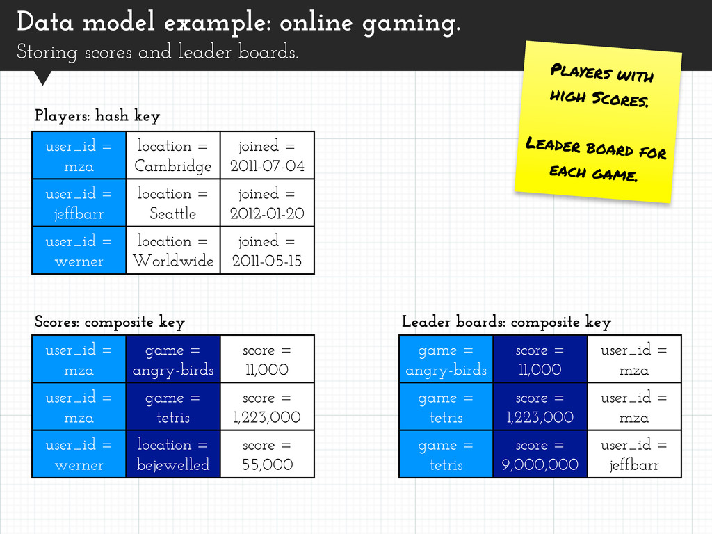
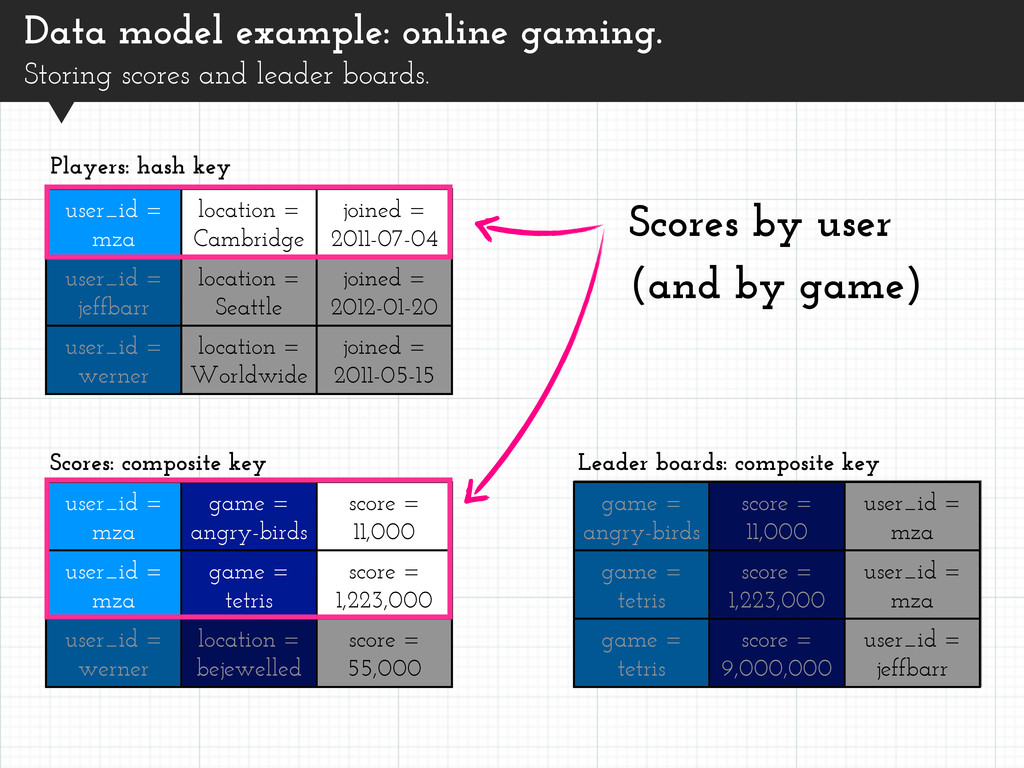
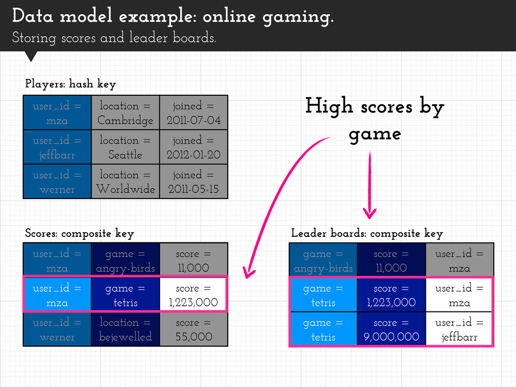
Players with high Scores. Leader board for each game. user_id = mza location = Cambridge joined = 2011-07-04 user_id = jeffbarr location = Seattle joined = 2012-01-20 user_id = werner location = Worldwide joined = 2011-05-15 Players: hash key
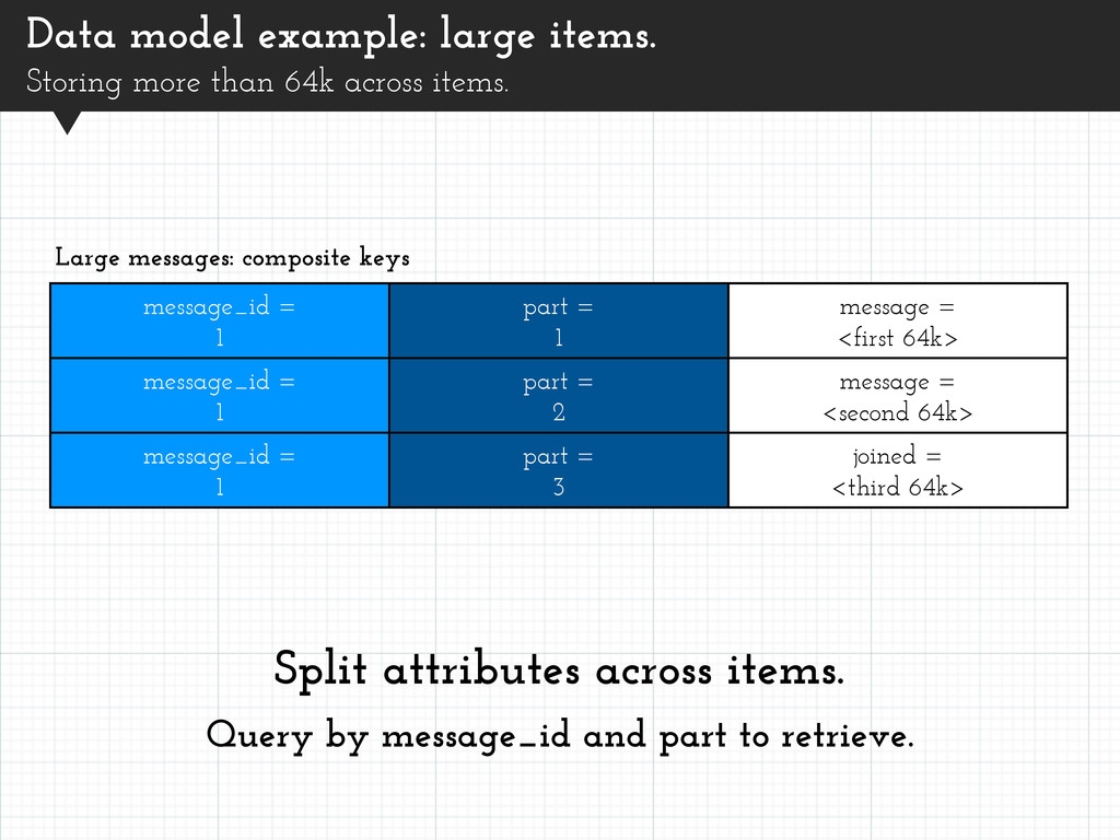
items. message_id = 1 part = 1 message = <first 64k> message_id = 1 part = 2 message = <second 64k> message_id = 1 part = 3 joined = <third 64k> Large messages: composite keys Split attributes across items. Query by message_id and part to retrieve.
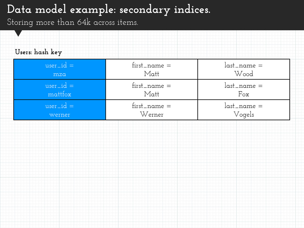
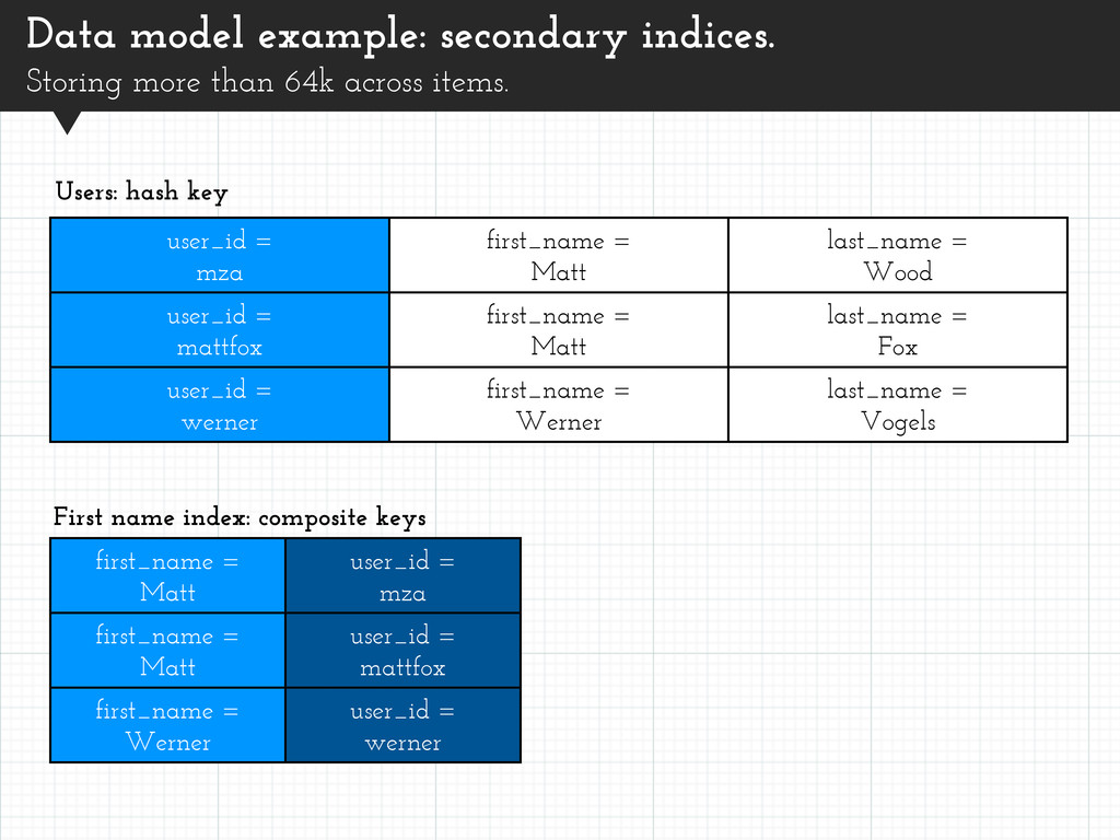
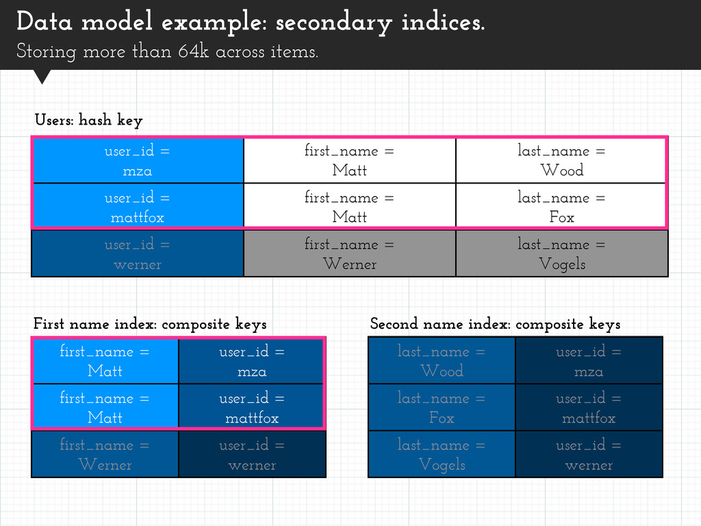
items. user_id = mza first_name = Matt last_name = Wood user_id = mattfox first_name = Matt last_name = Fox user_id = werner first_name = Werner last_name = Vogels Users: hash key first_name = Matt user_id = mza first_name = Matt user_id = mattfox first_name = Werner user_id = werner First name index: composite keys
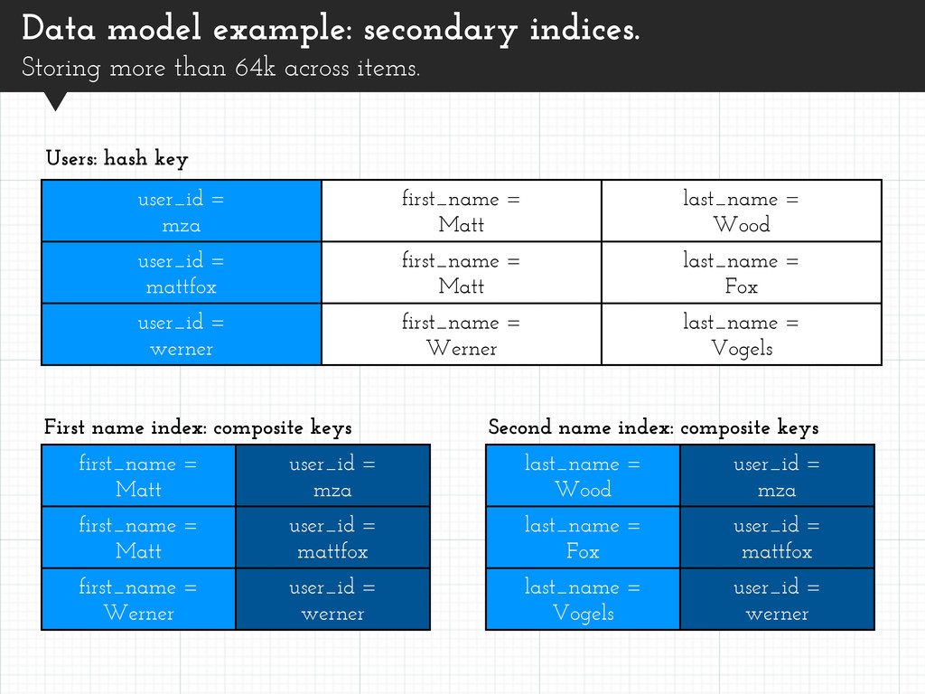
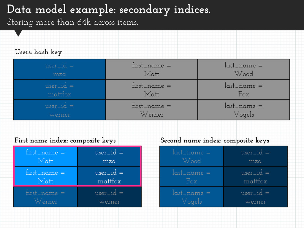
= mattfox last_name = Vogels user_id = werner user_id = mza first_name = Matt last_name = Wood user_id = mattfox first_name = Matt last_name = Fox user_id = werner first_name = Werner last_name = Vogels Data model example: secondary indices. Storing more than 64k across items. Users: hash key first_name = Matt user_id = mza first_name = Matt user_id = mattfox first_name = Werner user_id = werner First name index: composite keys Second name index: composite keys
= mattfox last_name = Vogels user_id = werner user_id = mza first_name = Matt last_name = Wood user_id = mattfox first_name = Matt last_name = Fox user_id = werner first_name = Werner last_name = Vogels Data model example: secondary indices. Storing more than 64k across items. Users: hash key first_name = Matt user_id = mza first_name = Matt user_id = mattfox first_name = Werner user_id = werner First name index: composite keys Second name index: composite keys
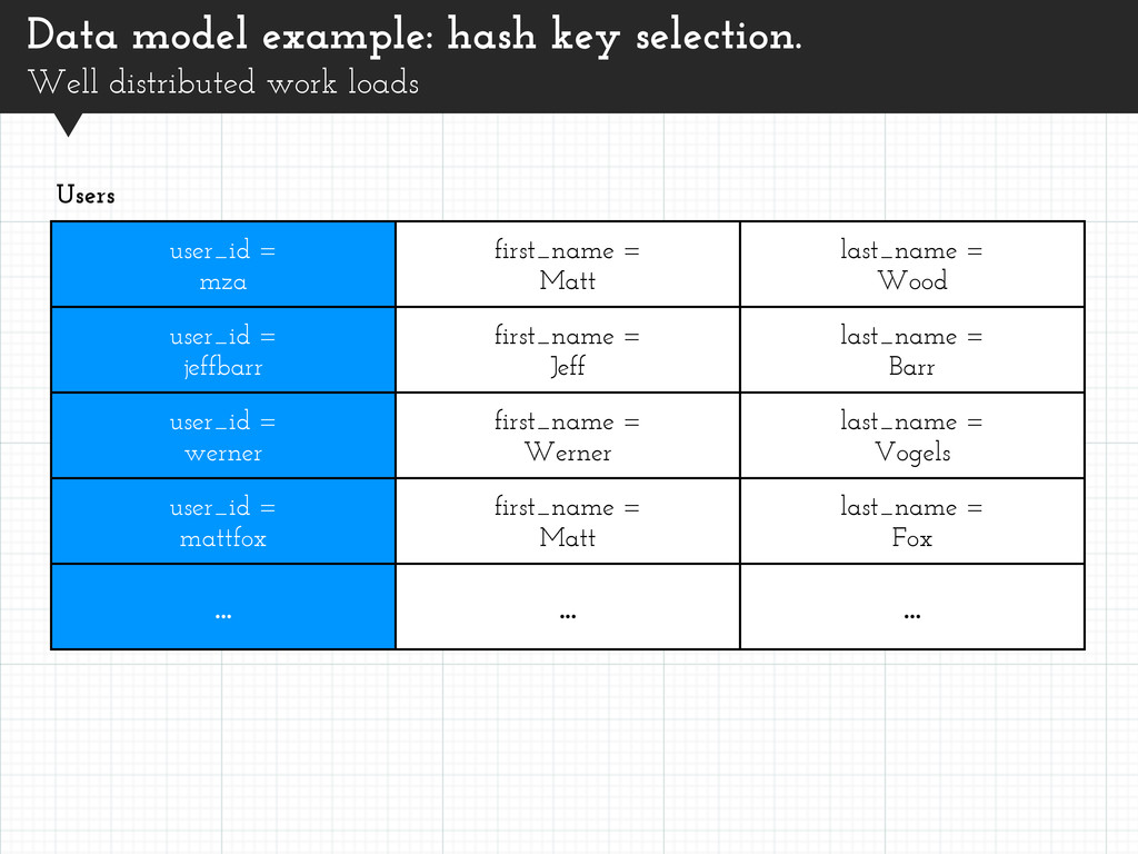
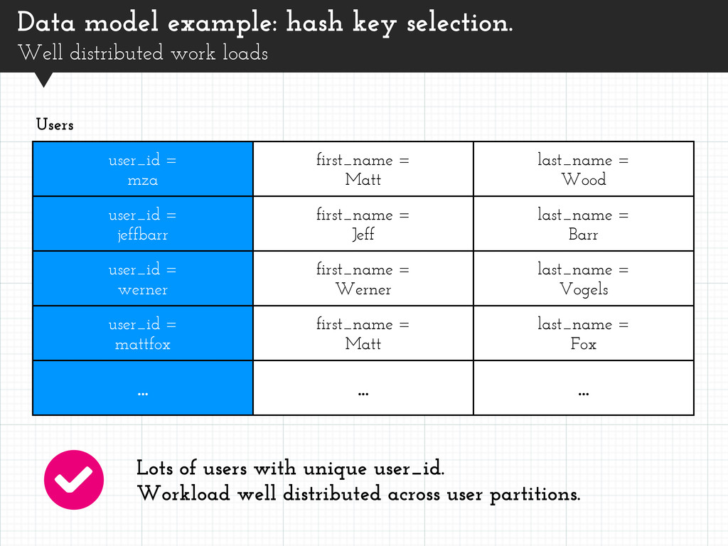
user_id = mza first_name = Matt last_name = Wood user_id = jeffbarr first_name = Jeff last_name = Barr user_id = werner first_name = Werner last_name = Vogels user_id = mattfox first_name = Matt last_name = Fox ... ... ... Users Lots of users with unique user_id. Workload well distributed across user partitions.
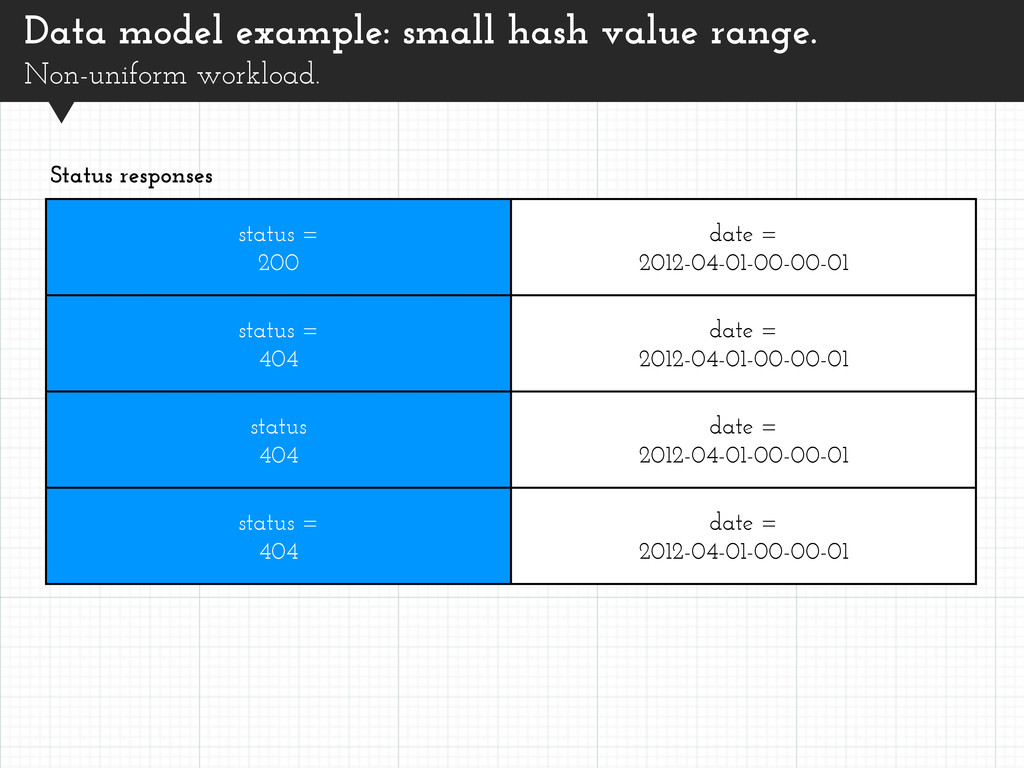
= 200 date = 2012-04-01-00-00-01 status = 404 date = 2012-04-01-00-00-01 status 404 date = 2012-04-01-00-00-01 status = 404 date = 2012-04-01-00-00-01 Status responses
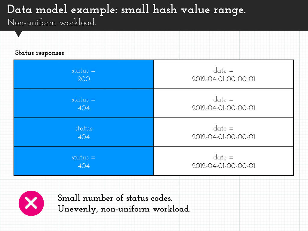
= 200 date = 2012-04-01-00-00-01 status = 404 date = 2012-04-01-00-00-01 status 404 date = 2012-04-01-00-00-01 status = 404 date = 2012-04-01-00-00-01 Status responses Small number of status codes. Unevenly, non-uniform workload.
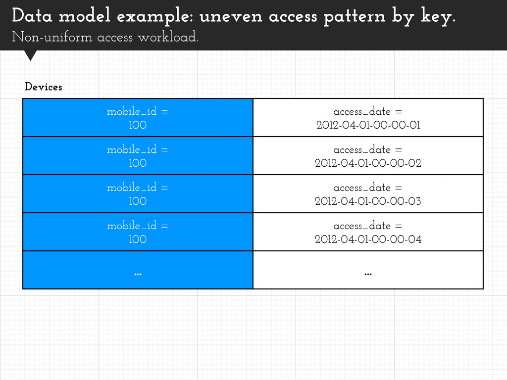
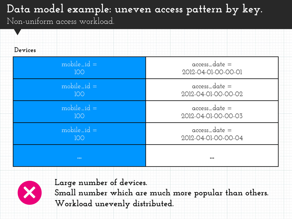
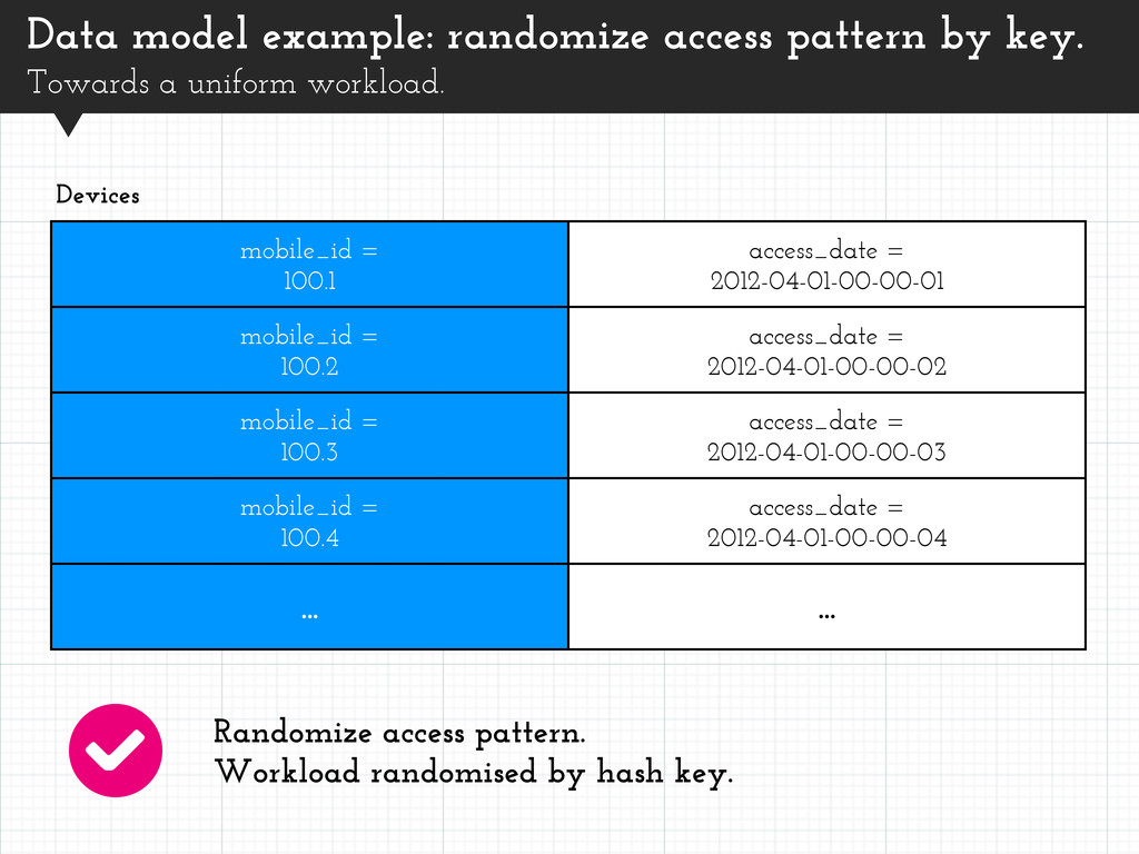
= 2012-04-01-00-00-02 mobile_id = 100 access_date = 2012-04-01-00-00-03 mobile_id = 100 access_date = 2012-04-01-00-00-04 ... ... Devices Large number of devices. Small number which are much more popular than others. Workload unevenly distributed. Data model example: uneven access pattern by key. Non-uniform access workload.
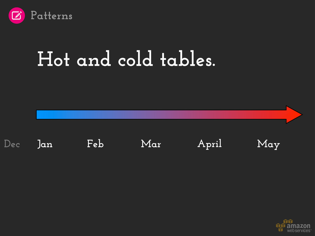
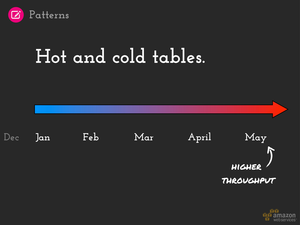
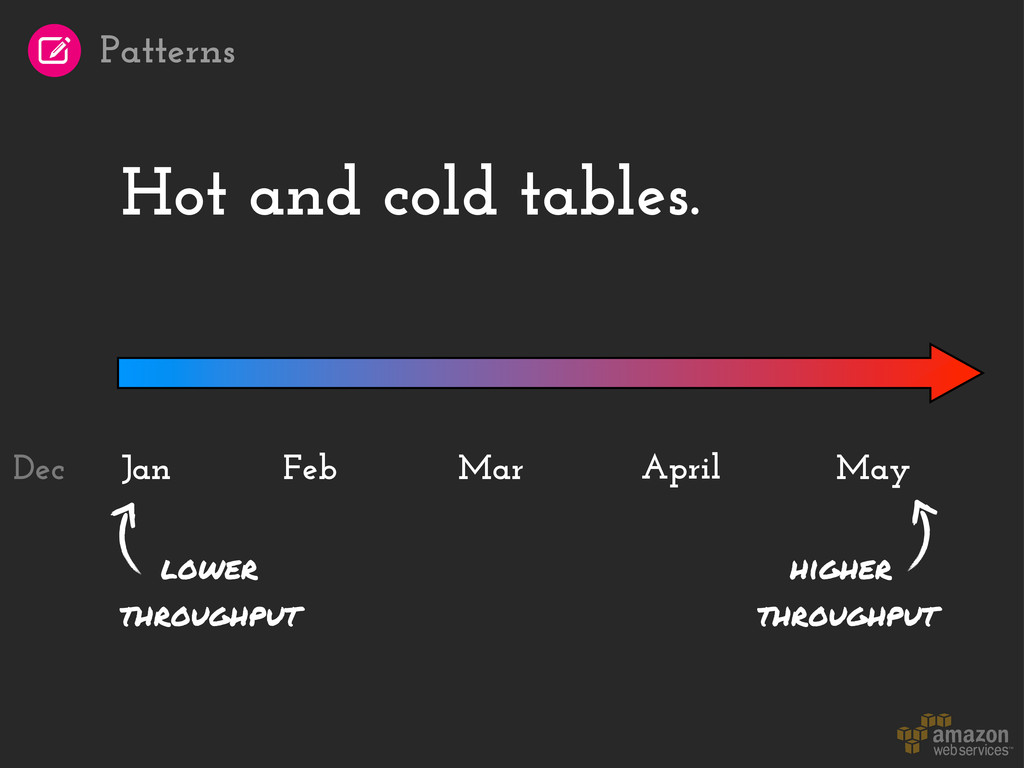
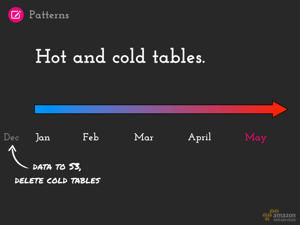
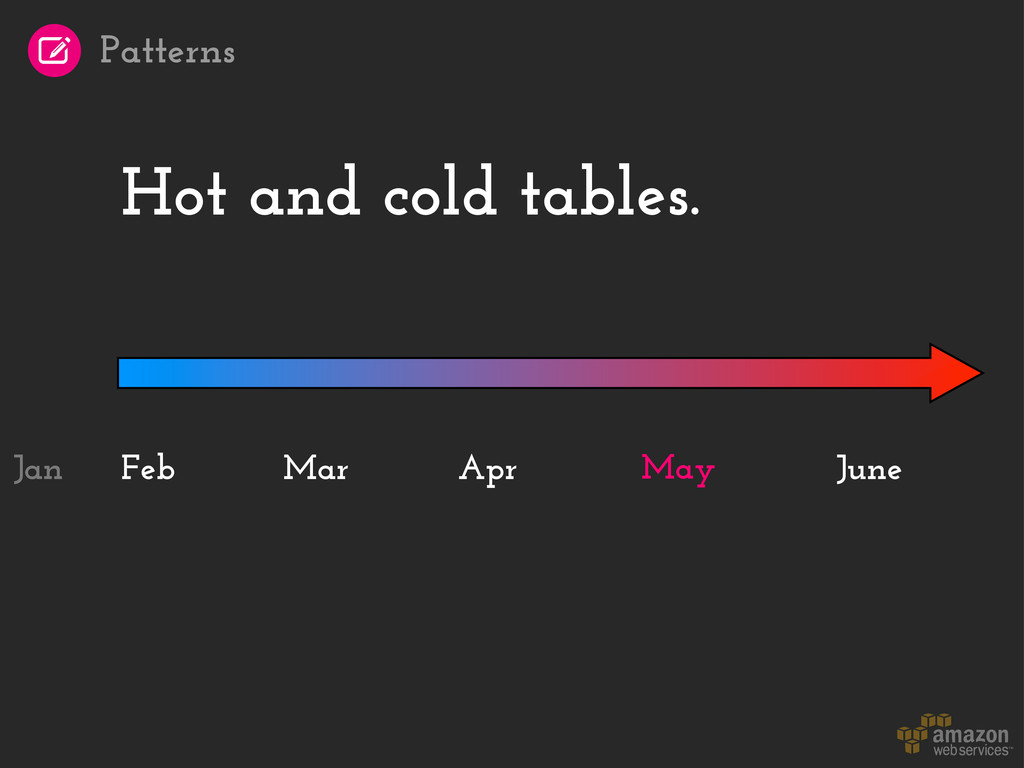
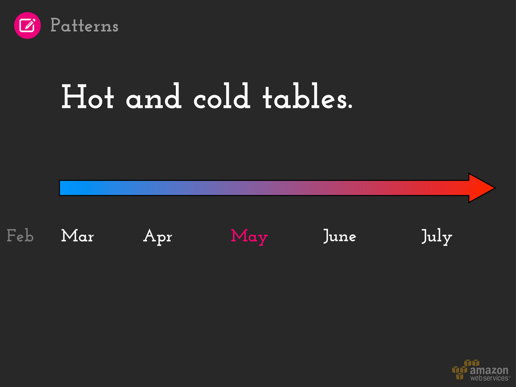
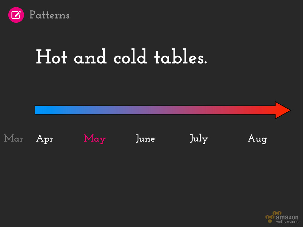
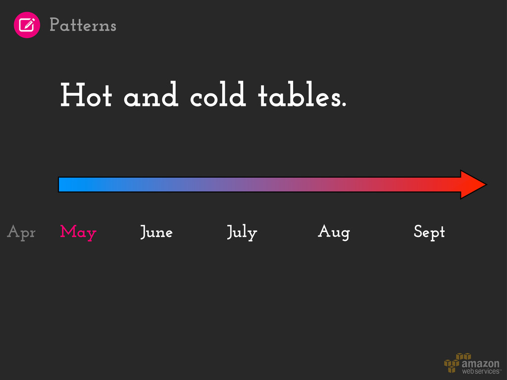
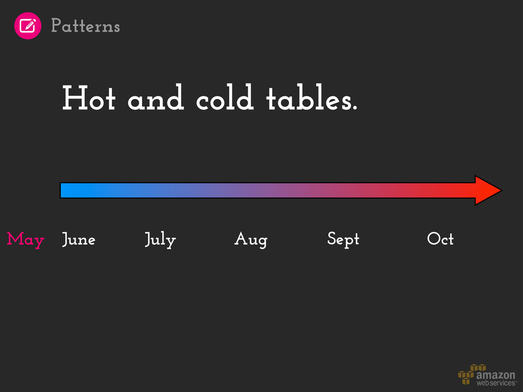
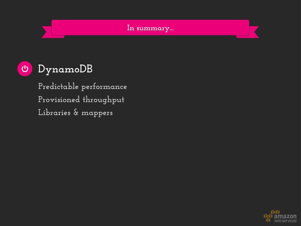
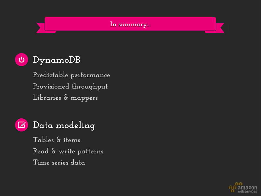
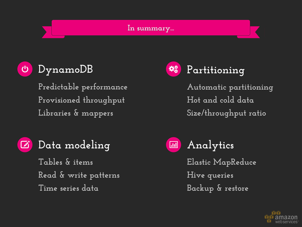
throughput Libraries & mappers Tables & items Read & write patterns Time series data Automatic partitioning Hot and cold data Size/throughput ratio Elastic MapReduce Hive queries Backup & restore
![Q & A [email protected] @mza](https://files.speakerdeck.com/presentations/4fb43700cef64e001f00cdbf/slide_128.jpg)