LQR Learning Pipelines

Transcript

1. LQR Learning Pipelines between reinforcement learning & adaptive control Florian Dörfler, ETH Zürich IEEE 14th Data Driven Control and Learning Systems Conference, Wuxi, China, 2025 1
2. Acknowledgments Pietro Tesi (Florence) Alessandro Chiuso (Padova) Claudio de Persis (Groningen) A. V. Papadopoulos (Uppsala) Feiran Zhao 赵斐然 (ETH Zürich) Keyou You 游科友 (Tsinghua) Linbin Huang 黄林彬 (Zhejiang) Xuerui Wang (Delft) Further: Roy Smith, Niklas Persson, Andres Jürisson, & Mojtaba Kaheni → papers 2
3. PERSPECTIVES ON DATA-DRIVEN CONTROL 3
4. Scientific landscape Rich & vast history (auto-tuners ‘79) fragmented between fields: adaptive control & reinforcement learning (RL) Culture gaps: adaptive control RL • stabilization vs online optimization • robust vs optimism facing uncertainty • interpretable pen+paper vs compute • theory certificates vs empirical studies • common root: dynamic programming • early cross-overs: neuro/adaptive DP • today: cross-fertilization & bridging culture gaps 4
5. Data-driven pipelines • direct (model-free) approach: MFAC, direct MRAC, behavioral, … ID • episodic & batch algorithms: collect data batch → design policy • online & adaptive algorithms: measure → update policy → act → gold standard: adaptive + optimal + robust + cheap + tractable …& direct • indirect (model-based) approach: data → model + uncertainty → control well-documented trade-offs • goal: optimality vs robust stability • practicality: modular vs end-to-end • complexity: data, compute, theory 5
6. • cornerstone & the benchmark of both optimal + adaptive control & RL • research gaps: no direct + adaptive LQR & no closed-loop certificates of adaptive DP methods Back to basics: LQR minimize 𝐾 𝔼𝑤𝑡 lim 𝑇→∞ 1 𝑇 σ𝑡=0 𝑇 𝑥𝑡 𝑇𝑄𝑥𝑡 + 𝑢𝑡 𝑇𝑅𝑢𝑡 s. t. 𝑥+ = 𝐴𝑥 + 𝐵𝑢 + 𝑤 𝑢 = 𝐾 𝑥 • 𝛨2 parameterization of LQR direct indirect offline batch online adaptive ? 𝑥 𝑢 𝑥+ = 𝐴𝑥 + 𝐵𝑢 + 𝑤 𝑧 = 𝑄1/2𝑥 + 𝑅1/2𝑢 𝑢 = 𝐾𝑥 𝑧 𝑤 6
7. Today: revisit old problems with new perspectives ① Behavior: a linear system is a sub- space of trajectories that can be re- presented by models or data: trajectory matrices or sample covariances 𝑥 ② adaptation of optimal control following RL-style policy gradient descent 𝐾+= 𝐾 − 𝜂 ∇𝐽 𝐾 𝐾+ 𝐾 7 [plot: Zheng, Pai, Tang]
8. Contents 1. problem setup for adaptive LQR via policy gradient 2. learning pipelines for (in)direct policy gradients 3. closed loop: sequential stability, optimality, & robustness 4. case studies: numerics, robotics, flight, & power systems 8
9. PROBLEM SETUP FOR ADAPTIVE LQR VIA POLICY GRADIENT 9
10. Policy parameterization min 𝐾 𝔼𝑤𝑡 lim 𝑇→∞ 1 𝑇 σ𝑡=0 𝑇 𝑥𝑡 𝑇𝑄𝑥𝑡 + 𝑢𝑡 𝑇𝑅𝑢𝑡 s. t. 𝑥+ = 𝐴𝑥 + 𝐵𝑢 + 𝑤 𝑢 = 𝐾 𝑥 → with controllability Gramian or state covariance Σ = lim 𝑇→∞ σ𝑡=0 𝑇 𝑥𝑡𝑥𝑡 𝑇 𝑇 min 𝐾,Σ≻0 𝑇𝑟 𝑄Σ) + 𝑇𝑟(𝐾𝑇𝑅𝐾Σ s. t. Σ = 𝐼 + 𝐴 + 𝐵𝐾 Σ 𝐴 + 𝐵𝐾 𝑇 → algorithmics: reformulation as SDP or discrete Riccati equation solved by interior point, contraction, or policy evaluation/improvement 𝑥 𝑢 𝑥+ = 𝐴𝑥 + 𝐵𝑢 + 𝑤 𝑧 = 𝑄1/2𝑥 + 𝑅1/2𝑢 𝑢 = 𝐾𝑥 𝑧 𝑤 10
11. • collect data (𝑋0 , 𝑈0 , 𝑋1 ) with 𝑊0 unknown & PE: rank 𝑈0 𝑋0 = 𝑛 + 𝑚 • indirect & certainty- equivalence LQR (all solved offline) least squares SysID certainty- equivalent LQR Indirect & certainty-equivalence LQR min 𝐾,Σ≻0 𝑇𝑟 𝑄Σ) + 𝑇𝑟(𝐾𝑇𝑅𝐾Σ s. t. Σ = 𝐼 + መ 𝐴 + ෠ 𝐵𝐾 Σ መ 𝐴 + ෠ 𝐵𝐾 𝑇 ෠ 𝐵, መ 𝐴 = arg min 𝐵,𝐴 𝑋1 − 𝐵, 𝐴 𝑈0 𝑋0 𝐹 11
12. • shortcoming of separating offline learning & online control → cannot improve policy online & cheaply / rapidly adapt • • desired adaptive solution: online (non-episodic / batch) algorithm, with closed-loop data, recursive implementation, & (in?)direct • how to “best” improve policy online → go down the gradient ! PII: S0005–1098(98)00089–2 Automatica, Vol. 34, No. 10, pp. 1161— 1167, 1998 IFAC. Published by Elsevier Scienc All rights reserved. Printed in Great B 0005-1098/98 $—see front m Adaptive Control: Towards a Complexity-Based General Theory* G. ZAM ES- Key Words—H control; adaptive control; learning control; performance analysis. Abstract—Two recent developments are pointing the way to- wards an input— output theory of H ! l adaptive feedback: The solution of problems involving: (1) feedback performance exact optimization under large plant uncertainty on the one hand (thetwo-disc problem of H ); and (2) optimally fast identi- fication in H on the other. Taken together, these are yielding adaptive algorithms for slowly varying data in H ! l . At a conceptual level, theseresultsmotivatea general input— output theory linking identification, adaptation, and control learning. In such a theory, thedefinition of adaptation isbased on system performance under uncertainty, and is independent of internal structure, presence or absence of variable parameters, or even feedback. 1998 IFAC. Published by Elsevier Science Ltd. All rights reserved. 1. INTRODUCTION What should the terms ‘‘adaptive’’ and ‘‘learning’’ mean in the context of control?Is it possibleto tell whether or not a black box is adaptive without certain difficulties. Controllers with ident external behavior can have an endless vari of parametrizations; variable parameters in o parametrization may be replaced by a fixed pa meter nonlinearity in another. In most of therec control literature there is no clear separation tween the concepts of adaptation and nonlin feedback, or between research on adaptive cont and nonlinear stability. This lack of clarity exten to fields other than control; e.g. in debates as whether neural nets do or do not have a learn capacity;or in theclassical 1960sChomsky vsSk ner argument as to whether children’s langu skills arelearned from theenvironment tabula r style, or to a largeextent are‘‘built in’’. (How co one tell the difference anyway?). It can be argu that the lack of a conceptual framework for ad * disclaimer: a large part of the adaptive control community focuses on stability & not optimality monotonicity principles of adaptive control: acquire information & im- prove control performance over time Towards an online & adaptive implementation 12
13. Adaptive LQR via policy gradient descent 𝑥+ = 𝐴𝑥 + 𝐵𝑢 + 𝑤 𝐾+ = 𝐾 − 𝜂 ∇𝐽 𝐾 𝑥 𝑢 𝐾𝑥 plant control policy 𝑤 policy gradient descent 𝑧 Seems obvious but… → algorithms • how to compute ∇𝐽 𝐾 cheaply & recursively ? • direct or indirect ? • convergence ? → closed loop • stability ? • robustness ? • optimality ? gradient of LQR cost as a function of 𝐾 + probing noise 13
14. Preview: does it work on an autonomous bike ? autonomous bike 𝐾+ = 𝐾 − 𝜂 ∇𝐽 𝐾 𝑢 = 𝐾𝑥 𝑤 𝑧 + feedback linearization adaptive control via policy gradient pre-stabilized plant Setup: autonomous bicycle with coarse inner control (2d dynamics stabilized by feedback linearization) & outer adaptive policy gradient + probing noise 14
15. LEARNING PIPELINES FOR POLICY GRADIENT 15
16. Algorithmic road map data sample covariance model identification indirect direct Hewer algorithm Newton metric policy gradient vanilla regularization robust gradient … … … regularization vanilla Newton metric natural gradient Fisher metric Fisher metric 16
17. Algorithmic road map data sample covariance model identification indirect direct Hewer algorithm Newton metric policy gradient vanilla regularization robust gradient … … … regularization vanilla Newton metric natural gradient Fisher metric Fisher metric 17
18. LQR optimization landscape min 𝐾,Σ≻0 𝑱 𝑲 = 𝑇𝑟 𝑄Σ) + 𝑇𝑟(𝐾𝑇𝑅𝐾Σ s. t. Σ = 𝐼 + 𝐴 + 𝐵𝐾 Σ 𝐴 + 𝐵𝐾 𝑇 after eliminating unique 𝚺 ≻ 𝟎, denote the objective as 𝑱 𝑲 • differentiable with ∇𝐽 𝐾 = 2 𝑅 + 𝐵𝑇𝑃 𝐵 𝐾 − 𝐵𝑇𝑃𝐴 Σ where 𝑃 = 𝑄 + 𝐾𝑇𝑅𝐾 + 𝐴 + 𝐵𝐾 𝑇𝑃 𝐴 + 𝐵𝐾 & Σ are closed-loop obs. + contr. Gramians • coercive with compact sublevel sets • smooth with locally bounded Hessian • gradient dominance: 𝐽 𝐾 ≤ 𝐽∗ + 𝑐𝑜𝑛𝑠𝑡. ∙ ∇𝐽 𝐾 2 𝐽 𝐾 is usually not convex 18 but for stabilizing 𝐾 is [plot: Zheng, Pai, Tang]
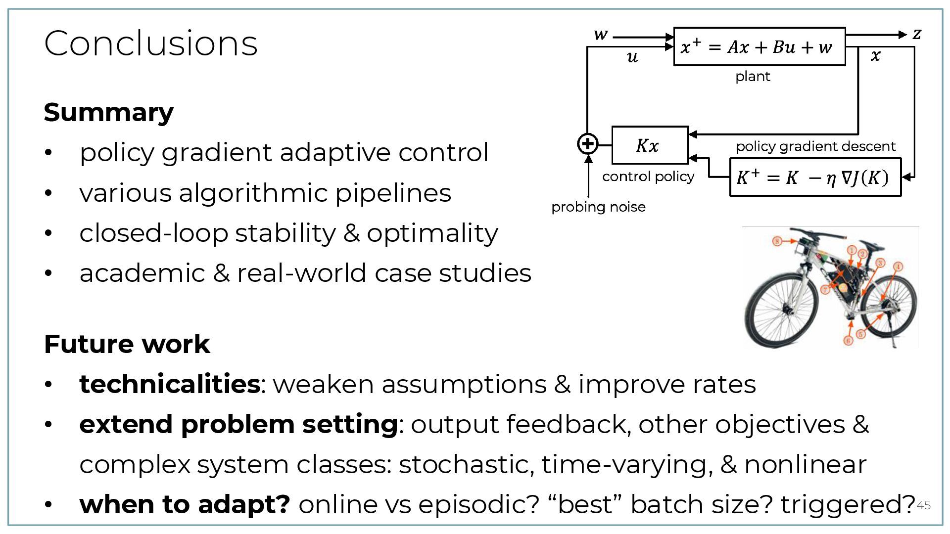
19. Model-based policy gradient min 𝐾 𝐽 𝐾 = 𝑇𝑟 𝑄Σ) + 𝑇𝑟(𝐾𝑇𝑅𝐾Σ Annual Review of Control, Robotics , and AutonomousSys tems Toward aT heoretical Foundation of Policy Optimization for Learning Control Policies Bin Hu,1 Kaiqing Zhang,2,3 Na Li,4 Mehran Mesbahi,5 Maryam Fazel,6 and Tamer Ba¸ sar1 1Coordinated Science Laboratory and Department of Electrical and Computer Engineering, University of Illinois Urbana-Champaign, Urbana, Illinois, USA; email: binhu7@ illinois.edu, basar1@ illinois.edu 2Laboratory for Information and Decision Systems and Computer Science and Artif cial Intelligence Laboratory, Massachusetts Institute of Technology, Cambridge, Massachusetts, USA 3Current aff liation: Department of Electrical and Computer Engineering and Institute for Systems Research, University of Maryland, College Park, Maryland, USA; email: kaiqing@ umd.edu 4School of Engineering and Applied Sciences, Harvard University, Cambridge, Massachusetts, USA; email: nali@ seas.harvard.edu 5Department of Aeronautics and Astronautics, University of Washington, Seattle, Washington, USA; email: mesbahi@ uw.edu 6Department of Electrical and Computer Engineering, University of Washington, Seattle, Washington, USA; email: mfazel@ uw.edu Annu. Rev. Control Robot. Auton. Syst. 2023. 6:123–58 T he Annual Review of Control, Robotics , and AutonomousSystemsisonline at control.annualreviews.org https://doi.org/10.1146/annurev-control-042920- 020021 Copyright © 2023 by the author(s). T his work is licensed under aCreative Commons Attribution 4.0 International License, which permits unrestricted use, distribution, and reproduction in any medium, provided the original author and source are credited. See credit lines of images or other third-party material in this article for license information. Keywords policy optimization, reinforcement learning, feedback control synthesis Abstract Gradient-based methodshave been widely used for system design and opti- mization in diverse application domains. Recently, there hasbeen arenewed interest in studying theoretical propertiesof thesemethodsin thecontext of control and reinforcement learning. T hisarticle surveyssome of the recent developments on policy optimization, a gradient-based iterative approach for feedback control synthesis that hasbeen popularized by successesof re- inforcement learning. We take an interdisciplinary perspective in our expo- sition that connects control theory, reinforcement learning, and large-scale Fact: For initial 𝐾0 stabilizing & small 𝜂, gradient descent 𝐾+ = 𝐾 − 𝜂 ∇𝐽 𝐾 converges linearly to 𝐾∗. where Σ = 𝐼 + 𝐴 + 𝐵𝐾 Σ 𝐴 + 𝐵𝐾 𝑇 Algorithm: model-based adaptive control via policy gradient 1. data collection: refresh (𝑋0 , 𝑈0 , 𝑋1 ) 2. identification of ෠ 𝐵, መ 𝐴 via recursive LS 3. policy gradient: 𝐾+ = 𝐾 − 𝜂 ∇𝐽 𝐾 using estimates ෠ 𝐵, መ 𝐴 & closed-loop Gramians Σ, 𝑃 actuate & repeat 19
20. Algorithmic road map data sample covariance model identification indirect direct Hewer algorithm policy gradient vanilla regularization robust gradient … … … regularization vanilla Newton metric natural gradient Newton metric Fisher metric Fisher metric 20
21. Pre-scaled policy gradient 𝐾+ = 𝐾 − 𝜂 𝑴(𝑲) ∇𝐽 𝐾 Fact: this equals Hewer’s algorithm: policy evaluation ⇆ improvement → Natural policy gradient method: 𝑴 𝐾 is inverse Fisher information −∇𝐽 𝐾 ≈ steepest descent in Euclidean metric − 𝑴 𝐾 ∇𝐽 𝐾 ≈ descent in direction with large variance Fact: 𝑴 𝐾 ∇𝐽 𝐾 = ∇𝐽 𝐾 Σ−1 is easy to evaluate → Gauss-Newton: 𝑴(𝑲) cheaply approximates inverse Hessian ∇2𝐽 𝐾 21
22. Algorithmic road map data sample covariance model identification indirect direct Hewer algorithm policy gradient vanilla regularization robust gradient … … … regularization vanilla Newton metric natural gradient Newton metric Fisher metric Fisher metric 22
23. relative performance gap 𝜖 = 1 𝜖 = 0.1 𝜖 = 0.01 # trajectories (100 samples) 1414 43850 142865 ~ 𝟏𝟎𝟕 samples for 4th order system • issue: uncertainty propagation is hard in indirect case & outcome suffers from bias error (e.g. model-order in output feedback setup) • model-free 0th order methods constructing two-point estimate ෣ ∇𝐽(𝐾) = 𝐽 𝐾 + 𝑟𝑈 − 𝐽 𝐾 − 𝑟𝑈 ⋅ 𝑚𝑛 𝑟2 𝑈 from uniform perturbation 𝑈 & numerous + very long trajectories • direct policy gradient is inefficient, episodic, & practically useless ? → sample covariance parameterization to the rescue ! Direct (model-free) policy gradient methods 23
24. • sample covariances: Λ = 1 𝑡 𝑈0 𝑋0 𝑈0 𝑋0 ⊤ ≻ 0 & Λ+ = 1 𝑡 𝑋1 𝑈0 𝑋0 ⊤ • direct data-driven formulation by substituting 𝐴 + 𝐵𝐾 = Λ+V & (⋆) Behavioral sample covariance parametrization ⟹ ∀𝐾 ∃𝑉 s. t. 𝐾 𝐼 = 1 𝑡 𝑈0 𝑋0 𝑈0 𝑋0 ⊤ 𝑉 (⋆) 𝑋1 = 𝐴𝑋0 + 𝐵 𝑈0 𝑋0 = 𝑥0 , … , 𝑥𝑡−1 𝑈0 = 𝑢0 , … , 𝑢𝑡−1 𝑋1 = 𝑥1 , … , 𝑥𝑡 • closed loop: 𝐴 + 𝐵𝐾 = 𝐵 𝐴 𝐾 𝐼 = 𝐵 𝐴 1 𝑡 𝑈0 𝑋0 𝑈0 𝑋0 ⊤ V = 1 𝑡 𝑋1 𝑈0 𝑋0 ⊤ V (no noise) = Λ+V (due to PE) 24
25. Aside: covariance parametrization on the rise Related to trajectory matrices, but • matrices independent of data size • uniqueness & no regularization • recursive rank-1 updates 25
26. Covariance parametrization of policy gradient • covariance parameterization: substitute 𝐴 + 𝐵𝐾 = Λ+V with linear constraint 𝐾 𝐼 = Λ 𝑉 • analogous optimization problem in 𝑉-coordinates with linear constraint, where 𝐾 can be eliminated • direct & projected policy gradient 𝑉+ = 𝑉 − 𝜂 Π ∇𝐽 𝑉 case study: random 4th order system & only 6 data samples min 𝐾,Σ≻0,𝑉 𝑇𝑟 𝑄Σ) + 𝑇𝑟(𝐾𝑇𝑅𝐾Σ s. t. Σ = 𝐼 + Λ+𝑉 Σ Λ+𝑉 𝑇 𝐾 𝐼 = Λ 𝑉 26 optimality gap
27. Facts on direct policy gradient • covariance parameterization: substitute 𝐴 + 𝐵𝐾 = Λ+V with 𝐾 𝐼 = Λ 𝑉 • direct & projected policy gradient descent 𝑉+ = 𝑉 − 𝜂 Π ∇𝐽 𝑉 Fact 1: in original 𝐾 −coordinates reads as scaled gradient descent 𝐾+ = 𝐾 − 𝜂 𝑴𝒕 ∇𝐽 𝐾 , where 𝑴𝒕 = 1 𝑡2 𝑈0 𝑈0 𝑋0 ⊤ Π 𝑈0 𝑋0 𝑈0 𝑇≻ 0 . → retain strong convergence result Fact 2: the corresponding natural gradient descent is invariant, i.e., equal to the model-based natural gradient descent. → recover original result 27
28. Algorithmic road map data sample covariance model identification indirect direct Hewer algorithm policy gradient vanilla regularization robust gradient … … … regularization vanilla Newton metric natural gradient Newton metric Fisher metric Fisher metric robust gradient to counter noise 28
29. Robustifying covariance regularization of the LQR 𝑋1 = 𝐴𝑋0 + 𝐵 𝑈0 + 𝑊0 𝑋0 = 𝑥0 , … , 𝑥𝑡−1 𝑈0 = 𝑢0 , … , 𝑢𝑡−1 𝑋1 = 𝑥1 , … , 𝑥𝑡 𝑊0 = 𝑤0 , … , 𝑤𝑡−1 • closed loop: 𝐴 + 𝐵𝐾 = Λ+ − ෩ 𝑊0 𝑉 where ෩ 𝑊0 = 1 𝑡 𝑊0 𝑈0 𝑋0 ⊤ (neglected before) • difference in Lyapunov equn’s with/without noise ~ 𝑽𝚺𝑽𝑻𝚲 • regularized LQR: 𝐽 𝑉 + 𝜆 ⋅ 𝑇𝑟 𝑽𝚺𝑽𝑻𝚲 = 𝐽 𝐾 + 𝜆 ⋅ 𝑇𝑟 𝚲−𝟏 𝑲 𝑰 𝚺 𝑲 𝑰 𝑻 • optimization class does not change → retain convergence result 29
30. Effect of regularization Comparison of stability % 𝑃 & median optimality gap ℳ optimality gap [%] median optimality gap [%] stabilizing controllers [%] • regularizing with 𝜆 robustifies & gives better performance • improves algorithmic stability for indirect & direct methods • decrease 𝜆 as data grows 30
31. CLOSED-LOOP STABILITY, OPTIMALITY & ROBUSTNESS 31
32. Policy gradient descent in closed loop 𝑥+ = 𝐴𝑥 + 𝐵𝑢 + 𝑤 𝐾+ = 𝐾 − 𝜂 𝑀 ∇𝐽 𝐾 𝑥 𝐾𝑥 plant control policy 𝑤 policy gradient descent 𝑧 gradient of LQR cost as a function of 𝐾 or any of previous policy gradient descent methods + probing noise 𝑢 = 𝐾𝑥 𝑒 Q: if each 𝐾𝑡 is stabilizing & 𝐽(𝐾𝑡 ) decreases, we surely get asymptotic stability & optimality ? A: it’s a switched system, ... so no ? 32 + 𝑒
33. Information metric • bounded noise covariance: 1 𝑡 𝑊0 𝑊0 𝑇 ≤ 𝛿𝑡 2 for some 𝛿𝑡 ≥ 0 • persistency of excitation due to probing: 𝜎 Λt ≥ 𝛾𝑡 2 for some 𝛾𝑡 ≥ 0 • information metric = signal-to-noise ratio 𝑆𝑁𝑅𝑡 ≔ Τ 𝛾𝑡 𝛿𝑡 Uniform 𝛿𝑡 ∼ 𝑂(1) Constant 𝛾𝑡 ∼ 𝑂(1) 𝑆𝑁𝑅𝑡 ∼ 𝑂(1) Gaussian 𝛿𝑡 ∼ 𝑂(1/ 𝑡) Constant 𝛾𝑡 ∼ 𝑂(1) 𝑆𝑁𝑅𝑡 ∼ 𝑂( 𝑡) Decay 𝛾𝑡 ∼ 𝑂(𝑡−1/4) 𝑆𝑁𝑅𝑡 ∼ 𝑂(𝑡1/4) satisfies Zames’ first monotonicity principle: information acquisition = SNR increases 33 PII: S0005–1098(98)00089–2 Automatica, Vol. 34, No. 10, pp. 1161— 1167, 199 1998 IFAC. Published by Elsevier Science L All rights reserved. Printed in Great Brita 0005-1098/98 $—see front matt Adaptive Control: Towards a Complexity-Based General Theory* G. ZAM ES- Key Words—H control; adaptive control; learning control; performance analysis. Abstract—Two recent developments are pointing the way to- wards an input— output theory of H ! l adaptive feedback: The solution of problems involving: (1) feedback performance exact optimization under large plant uncertainty on the one hand (thetwo-disc problem of H ); and (2) optimally fast identi- fication in H on the other. Taken together, these are yielding adaptive algorithms for slowly varying data in H ! l . At a conceptual level, theseresultsmotivatea general input— output theory linking identification, adaptation, and control learning. In such a theory, thedefinition of adaptation isbased on system performance under uncertainty, and is independent of internal structure, presence or absence of variable parameters, or even feedback. 1998 IFAC. Published by Elsevier Science Ltd. All rights reserved. 1. INTRODUCTION What should the terms ‘‘adaptive’’ and ‘‘learning’’ mean in the context of control?Is it possible to tell whether or not a black box is adaptive without knowledge of its internal structure? In design, is it possible to determine beforehand whether it is ne- cessary for a controller to adapt and learn in order to meet performance specifications, or is adapta- tion a matter of choice? In this overview we shall describe recent work in the H framework which provides a means of computing certain kinds of adaptive controllers, but which also sheds some light on these more conceptual questions. Despite the long history of research on adaptive control, and the considerable practical success of adaptive strategies associated with the names of certain difficulties. Controllers with identica external behavior can have an endless variet of parametrizations; variable parameters in on parametrization may be replaced by a fixed para meter nonlinearity in another. In most of therecen control literature there is no clear separation be tween the concepts of adaptation and nonlinea feedback, or between research on adaptive contro and nonlinear stability. This lack of clarity extend to fields other than control; e.g. in debates as t whether neural nets do or do not have a learnin capacity;or in theclassical 1960sChomsky vsSkin ner argument as to whether children’s languag skills arelearned from theenvironment tabula ras style, or to a largeextent are‘‘built in’’. (How coul one tell the difference anyway?). It can be argue that the lack of a conceptual framework for adap tive control has inhibited research in this area an made it difficult to compare alternative designs. We would like to re-examine these issues in th light of recent developments linking the theories o feedback, identification, complexity and time-vary ing optimization. The perspective here is actuall not new, having been outlined by theauthor on an off since the 1970s (Zames, 1976, 1979, 1981, 1989 However, the key mathematical details have bee worked out only recently, notably in joint wor with Lin et al. (Lin et al., 1992; Zames and Wang
34. Certificate for any of the policy gradient methods Theorem (simplified): There exist 𝜈𝑖 > 0, 𝑖 ∈ {1,2,3,4,5}, depending on 𝐴, 𝐵, 𝑄, 𝑅, 𝐾0 with 𝜈3 < 1, so that, if 𝑆𝑁𝑅𝑡 ≥ 𝜈1 ∀𝑡 , 𝜂 ≤ 𝜈2 , & for stable 𝐾0 1. the closed-loop system is stable in the sense that |𝑥𝑡 | ≤ 𝜈3 𝑡|𝑥0 | + 𝜈4 max 0≤𝑖<𝑡 |𝐵𝑒𝑖 + 𝑤𝑖 | . 2. the policy converges to optimality in the sense that 𝐶 𝐾𝑡 − 𝐶∗ ≤ 1 − 𝜂 𝜈5 𝑡 𝐶 𝐾𝑡0 − 𝐶∗ + 𝑂(𝑆𝑁𝑅𝑡 −1) nominal exponential convergence bias due to noise SNR & step-size requirements stable initialization 34
35. Notes on stability & convergence statement • assumptions: stable 𝐾0 + large enough SNR + small enough step size to control learning rate & assure sequential stability • convergence: nominal exponential + (decreasing) bias term → Zames’ 2nd monotonicity principle: improving performance → 𝑂 1/ 𝑡 for Gaussian noise & constant excitation → 𝑂 𝑡−1/4 for Gaussian noise & diminishing excitation • direct methods: 𝑆𝑁𝑅𝑡 ≥ 𝑐𝑜𝑛𝑠𝑡. 𝑀𝑡 𝜎 𝑀𝑡 , 𝜂𝑡 ≤ 𝑐𝑜𝑛𝑠𝑡. 𝑀𝑡 , & convergence rate depend on data-dependent matrix 𝑀𝑡 = 1 𝑡2 𝑈0 𝑈0 𝑋0 ⊤ Π 𝑈0 𝑋0 𝑈0 𝑇 slightly worse than optimal known rates 𝑂 1/𝑡 & 𝑂 1/ 𝑡 35
36. Notes on stability & convergence statement • all results also hold in regularized setting under proper choice of regularization coefficient 𝜆𝑡 ≤ 𝑂 (𝛾𝑡 𝛿𝑡 ) (const. for bounded noise) • Indirect Gauss-Newton method = adaptive version of Hewer’s algorithm, which needs additionally 𝐾0 sufficiently close to 𝐾∗ Algorithm: adaptive Hewer’s algorithm 1. data collection: refresh (𝑋0 , 𝑈0 , 𝑋1 ) 2. identification of ෠ 𝐵, መ 𝐴 via recursive LS 3. policy evaluation: 𝑃+ = Lyapynov ( ෠ 𝐵, መ 𝐴, 𝐾) 4. policy improvement: 𝐾+ = … −1𝑃+ ෠ 𝐵 መ 𝐴 actuate & repeat 36
37. Numerics: convergence to optimality • case study [Dean et al. ‘19]: discrete-time system with Gaussian noise 𝑤𝑡 ∈ 𝒩(0, 𝑖𝑑) • policy gradient methods are more robust to noise versus sensitive one-shot method • empirically observe tighter optimality gap ~ 𝑂(𝑆𝑁𝑅−2) than our certificate 𝑂(𝑆𝑁𝑅−1) optimality gap: mean ± std 37
38. Numerics: mean ± std of closed-loop realized cost data set #1 (quality data) data set #2 (poor data) → all converge with a bias, but one-shot & Gauss-Newton less robust 38
39. Numerics: computational efficiency → all policy gradient methods significantly outperform one-shot-based method in computational effort state dimension direct one-shot 39 running time (s) running time (s)
40. Implementations today 40
41. Power systems / electronics case study • wind turbine becomes unstable in weak grid → nonlinear oscillations • converter, turbine, & grid are black box for commission engineer • construct state space realization from time shifts (5ms sampling) of inputs & outputs → direct policy gradient synchronous generator & full-scale converter 41
42. probe & collect data oscillation observed activate policy gradient adaptative LQR control without DeePO with DeePO (100 iterations) with DeePO (1 iteration) time [s] without control adaptation with policy gradient adaptive control 42
43. change of system parameters (DC voltage setpoint & gain) AC grid voltage disturbance occurs time [s] without control adaptation with policy gradient adaptive control 43
44. CONCLUSIONS 44
45. Conclusions Summary • policy gradient adaptive control • various algorithmic pipelines • closed-loop stability & optimality • academic & real-world case studies Future work • technicalities: weaken assumptions & improve rates • extend problem setting: output feedback, other objectives & complex system classes: stochastic, time-varying, & nonlinear • when to adapt? online vs episodic? “best” batch size? triggered?45
46. THANKS 46