Drawing Heighway’s Dragon - Part II - Recursive Function Simplification - From 2^n Recursive Invocations To n Tail-Recursive Invocations Exploiting Self-Similarity

Drawing Heighway’s Dragon - Part II - Recursive Function Simplification - From 2^n Recursive Invocations To n Tail-Recursive Invocations Exploiting Self-Similarity.

Keywords: "heighway's dragon", "recursion", "tail-recursion", "graphics", "Scala", "functional programming", "self-similarity", "rotation", "translation", "matrix multiplication", "linear transformation"

Transcript

1. Drawing Heighway’s Dragon Recursive Function Simplification From 2n Recursive Invocations To n Tail-Recursive Invocations Exploiting Self-Similarity @philip_schwarz slides by https://fpilluminated.org/ Part 2 𝑥! 𝑦′ 1 = 𝑥 𝑦 1 𝐑 𝐑 = ? ? ? ? ? ? ? ? ?
2. In part 1 we looked at a Scala program that draws Heighway’s Dragon. At the heart of the program is the following recursive function used to grow a dragon path, which is a sequence of points: Once the path has been grown to the desired age, drawing the dragon amounts to drawing lines (of the given length) connecting consecutive pairs of the path’s points. On the right we see a drawing of a dragon aged 9. Thanks to its use of recursion, the function is very simple, yet it is far from obvious why its logic is able to compute a path that results in the aesthetically pleasing dragon pattern. extension (path: DragonPath) def grow(age: Int, length: Int, direction: Direction): DragonPath = def newDirections(direction: Direction): (Direction, Direction) = direction match case North => (West, North) case South => (East, South) case East => (East, North) case West => (West, South) path.headOption.fold(path): front => if age == 0 then front.translate(direction, length) :: path else val (firstDirection, secondDirection) = newDirections(direction) path .grow(age - 1, length, firstDirection) .grow(age - 1, length, secondDirection)
3. The first thing we want to do in part 2 is see if we can exploit the self-similarity of Heighway’s Dragon to simplify the grow function. While it is already very simple, we want to improve it further, so that it becomes simple to understand why it is able to accomplish its task. The way our program currently draws a dragon aged 𝑵 is by first computing a dragon path consisting of a sequence of 𝟐𝑵 + 𝟏 points 𝒑𝟏 , 𝒑𝟐 , …, 𝒑𝟐𝑵*𝟏 , and then drawing lines connecting each point 𝒑𝒊 with next point 𝒑𝒊*𝟏. Let us focus on how the program computes the path of a dragon aged N, not in terms of the exact steps taken by the program, but in terms of the following high level path-growing process: 1. start with a degenerate path consisting of a single point (the starting point) 2. .grow the path by computing a new point, and adding the latter to the front of the path 3. repeat the previous step until the path consists of 𝟐𝑵 + 𝟏 points. The next ten slides visualise the above process for a dragon aged 4. To make things easier to understand, rather than just visualising the addition of newly computed points, the slides also show lines connecting the points, as if lines get drawn at the same time as points are computed.
4. 𝑝1 Initially the path consists simply of starting point 𝒑𝟏 .
5. new point 𝑝2 is 𝑝1 translated East by distance length 𝑝1 𝑝2 > 1 ∶ 𝐸𝑎𝑠𝑡
6. > 2 ∶ 𝑁𝑜𝑟𝑡ℎ new point 𝑝3 is 𝑝2 translated North by distance length 𝑝1 𝑝2 𝑝3
7. new point 𝑝4 is 𝑝3 translated West by distance length 𝑝1 𝑝2 𝑝3 𝑝4 3 ∶ 𝑊𝑒𝑠𝑡
8. 𝑝1 𝑝2 𝑝3 𝑝4 > 𝑝5 4 ∶ 𝑁𝑜𝑟𝑡ℎ new point 𝑝5 is 𝑝4 translated North by distance length
9. 𝑝1 𝑝2 𝑝3 𝑝4 5 ∶ 𝑊𝑒𝑠𝑡 new point 𝑝6 is 𝑝5 translated West by distance length 𝑝5 𝑝6
10. 𝑝1 𝑝2 𝑝3 𝑝4 6 ∶ 𝑆𝑜𝑢𝑡ℎ new point 𝑝7 is 𝑝6 translated South by distance length 𝑝5 𝑝6 𝑝7
11. 𝑝1 𝑝2 𝑝3 𝑝4 new point 𝑝8 is 𝑝7 translated West by a distance length 𝑝5 𝑝6 𝑝7 7 ∶ 𝑊𝑒𝑠𝑡 𝑝8
12. 𝑝1 𝑝2 𝑝3 𝑝4 new point 𝑝9 is 𝑝8 translated North by a distance length 𝑝5 𝑝6 𝑝7 8 ∶ 𝑁𝑜𝑟𝑡ℎ 𝑝8 𝑝9 >
13. 𝑝1 𝑝2 𝑝3 𝑝4 𝑝5 𝑝6 𝑝7 𝑝8 𝑝9 > Here is the path computed by that process. Does the path exhibit any self-similarity? Are some parts of the path the same as other parts? Let’s find out in the next six slides.
14. There is no self-similarity in a dragon aged 0.
15. A dragon aged 1 exhibits self-similarity in that the second part of its path can be computed by taking the first part of the path, i.e. a dragon aged 0, and rotating it ninety degrees about the end point of the first part.
16. A dragon aged 2 also exhibits the same self-similarity: the second part of its path can be computed by taking the first part of the path, i.e. a dragon aged 1, and rotating it ninety degrees about the end point of the first part.
17. A dragon aged 3 again exhibits the same self-similarity: the second part of its path can be computed by taking the first part of the path, i.e. a dragon aged 2, and rotating it ninety degrees about the end point of the first part.
18. Let us now modify the high level path-growing process so that rather than computing the next point on a dragon path by translating the previously computed point (as seen below in the base case of the grow function), it instead computes new points on the path of a dragon aged N+1 by rotating the points on the path of a dragon aged N. extension (path: DragonPath) def grow(age: Int, length: Int, direction: Direction): DragonPath = def newDirections(direction: Direction): (Direction, Direction) = direction match case North => (West, North) case South => (East, South) case East => (East, North) case West => (West, South) path.headOption.fold(path): front => if age == 0 then front.translate(direction, length) :: path else val (firstDirection, secondDirection) = newDirections(direction) path .grow(age - 1, length, firstDirection) .grow(age - 1, length, secondDirection) The new process for a dragon aged N consists of phases 0 through to N-1. The next n slides visualise the new process for a dragon aged 4.
19. 𝑝1 𝑝2 > Phase 0 # of points: 2 = 20+1 # of lines: 1 = 20 We start off with two points
20. > 2 𝑝3 𝑝1 𝑝2 new point 𝑝3 is 𝑝1 rotated 90o about 𝑝2 > • iterate through the existing points on the path in reverse order • rotating each existing point so as to create a new point • which then becomes the ‘next’ point on the path In phase one there is only one existing point to process: 𝑝1 Phase 1
21. > 𝑝3 𝑝1 𝑝2 Phase 1 result # of points: 3 = 21+1 # of lines: 2 = 21
22. 3 𝑝3 𝑝1 𝑝2 new point 𝑝4 is 𝑝2 rotated 90o about 𝑝3 𝑝4 > 1st point • iterate through the existing points on the path in reverse order • rotating each existing point so as to create a new point • which then becomes the ‘next’ point on the path In phase two there are two existing points to process: 𝑝2 and 𝑝1 Phase 2
23. 4 𝑝1 new point 𝑝5 is 𝑝1 rotated 90o about 𝑝3 𝑝4 𝑝3 𝑝2 𝑝5 > 2nd point Phase 2
24. 𝑝1 𝑝4 𝑝3 𝑝2 𝑝5 > # of points: 5 = 22+1 # of lines: 4 = 22 Phase 2 result
25. 𝑝1 𝑝6 𝑝4 𝑝3 𝑝2 𝑝5 new point 𝑝6 is 𝑝4 rotated 90o about 𝑝5 > 5 1st point • iterate through the existing points on the path in reverse order • rotating each existing point so as to create a new point • which then becomes the ‘next’ point on the path In phase three there are four existing points to process: 𝑝4 , 𝑝3 , 𝑝2 , 𝑝1 Phase 3
26. 𝑝1 𝑝2 𝑝3 𝑝4 𝑝5 𝑝6 𝑝7 > 6 2nd point Phase 3 new point 𝑝7 is 𝑝3 rotated 90o about 𝑝5
27. 𝑝1 𝑝2 𝑝3 𝑝4 𝑝5 𝑝6 𝑝7 𝑝8 7 > 3rd point new point 𝑝8 is 𝑝2 rotated 90o about 𝑝5
28. 𝑝1 𝑝2 𝑝3 𝑝4 𝑝5 𝑝6 𝑝7 𝑝8 𝑝9 > > 4th point new point 𝑝9 is 𝑝1 rotated 90o about 𝑝5
29. 𝑝1 𝑝2 𝑝3 𝑝4 𝑝5 𝑝6 𝑝7 𝑝8 𝑝9 > # of points: 9 = 23+1 # of lines: 8 = 23 Phase 3 result
30. Because the new path-growing process computes new points simply by rotating existing points, the grow function no longer needs to concern itself with the concepts of direction and line length. Remember how the new process begins with two points? Direction and line length are now only needed to compute 𝒑𝟐 , when we create the initial dragon path. object DragonPath: def apply(startPoint: Point): DragonPath = List(startPoint) object DragonPath: def apply(startPoint: Point, direction: Direction, length: Int): DragonPath = val nextPoint = startPoint.translate(direction, distance = length) List(nextPoint, startPoint) extension (path: DragonPath) def grow(age: Int, length: Int, direction: Direction): DragonPath = def newDirections(direction: Direction): (Direction, Direction) = direction match case North => (West, North) case South => (East, South) case East => (East, North) case West => (West, South) <body of function – not shown> extension (path: DragonPath) def grow(age: Int): DragonPath = <new body of function – to be defined> Note that the apply function now returns List(nextPoint, startPoint). We have inverted the order of points in a path. Instead of new points being added to the end of the path, they will now new be added at the front of the path. We are doing this because it is more efficient to cons a new point onto a path than it is to append it to the end of the path. Doing so is legitimate because when the time comes to draw a line connecting points A and B, it makes no difference whether we draw a line from A to B or one from B to A.
31. Let’s update the Dragon’s path to reflect the improvements made on the previous slide. case class Dragon(start: Point, age: Int, length: Int, direction: Direction): val path: DragonPath = DragonPath(start) .grow(age, length, direction) case class Dragon(start: Point, age: Int, length: Int, direction: Direction): val path: DragonPath = DragonPath(start, direction, length) .grow(age)
32. extension (path: DragonPath) def grow(age: Int): DragonPath = <new body of function – to be defined> extension (path: DragonPath) @tailrec def grow(age: Int): DragonPath = if age == 0 || path.size < 2 then path else path.plusRotatedCopy.grow(age - 1) private def plusRotatedCopy: DragonPath = path.reverse.rotate(rotationCentre = path.head, angle = ninetyDegreesClockwise) ++ path val ninetyDegreesClockwise = -Math.PI / 2 Now it is time to reimplement the body of the grow function so that it exploits the dragon’s self-similarity. Instead of computing the next new point on a dragon path of age N by translating the last point on the path, it has to compute new points using the N-phase approach described earlier on, in which each phase involves the following steps: While the function remains recursive, it now becomes tail-recursive: instead of invoking itself twice, it invokes itself only once, that being the last thing it does. Rotation of the points on a dragon path around a rotation centre specified by another point is delegated to a function called rotate. • iterate through the existing points on the path in reverse order • rotating each existing point so as to create a new point • which then becomes the ‘next’ point on the path Now that the grow function exploits the dragon’s self-similarity, it is very easy to understand how the function accomplishes its task: to grow a path, first add to it a rotated copy of itself, and then recursively grow the resulting path. The rotation is centred on the point that was most recently added to the path. The angle of rotation is defined in radians, and is a negative value because a clockwise rotation is required, rather than the more customary, anti-clockwise one.
33. On the previous slide we saw that the grow function now delegates rotation of the points on a dragon path to a function called rotate. Here is its implementation: The function doesn’t do a lot. To rotate a number of points by a given angle (in radians) around a rotation centre specified by a point, it just delegates the rotation of each point to a second rotate function with the following signature: We’ll very soon be turning our attention to the implementation of this second rotate function. type Radians = Double extension (points: List[Point]) def rotate(rotationCentre: Point, angle: Radians): List[Point] = points.map(point => point.rotate(rotationCentre, angle)) def rotate(rotationCentre: Point, angle: Radians): Point
34. Now that we enjoy the benefit of having a plusRotatedCopy function whose intention-revealing name makes the exact details of its body less important for the purpose of quickly understanding how dragon paths are grown, it makes sense to make the function more efficient: instead of the function appending to the path a reversed and rotated copy of the path, it can use a left fold to avoid the append operation and do both the reversing and the rotation at the same time private def plusRotatedCopy = path.reverse.rotate(rotationCentre = path.head, angle = ninetyDegreesClockwise) ++ path private def plusRotatedCopy = path.foldLeft(path): (growingPath, point) => point.rotate(rotationCentre = path.head, angle = ninetyDegreesClockwise) :: growingPath
35. extension (path: DragonPath) def grow(age: Int, length: Int, direction: Direction): DragonPath = def newDirections(direction: Direction): (Direction, Direction) = direction match case North => (West, North) case South => (East, South) case East => (East, North) case West => (West, South) path.headOption.fold(path): front => if age == 0 then front.translate(direction, length) :: path else val (firstDirection, secondDirection) = newDirections(direction) path .grow(age - 1, length, firstDirection) .grow(age - 1, length, secondDirection) extension (path: DragonPath) @tailrec def grow(age: Int): DragonPath = if age == 0 || path.size < 2 then path else path.plusRotatedCopy.grow(age - 1) private def plusRotatedCopy = path.foldLeft(path): (growingPath, point) => point.rotate(rotationCentre = path.head, angle = ninetyDegreesClockwise) :: growingPath val ninetyDegreesClockwise = -Math.PI / 2 Here is a recap of how we changed the grow function.
36. A couple of slides ago we trivially implemented the rotate function that operates on a dragon path by getting it to delegate the rotation of a single point on that path to a second rotate function, with the following signature: How can we implement this function? Let’s consult Computer Graphics for Java Programmers and learn (or reacquaint ourselves with) just enough graphics-related mathematics to be able to implement the function. def rotate(rotationCentre: Point, angle: Radians): Point https://www.linkedin.com/in/leen-ammeraal-b97b968/ https://profiles.utdallas.edu/kang.zhang Leen Ammeraal Kang Zhang
37. Rotation of a point about the origin of a two-dimensional cartesian coordinate system is a linear transformation. A linear transformation maps a vector v to another vector v’. So the first concept that we need to be familiar with is that of a vector.
38. 2.1 Vectors … A vector is a directed line segment, characterized by its length and its direction only. Figure 2.1 shows two representations of the same vector 𝐚 = 𝐏𝐐 = 𝐛 = 𝐑𝐒. Thus a vector is not altered by a translation. The sum 𝒄 of the vectors 𝐚 and 𝐛, written 𝐜 = 𝐚 + 𝐛 can be obtained as the diagonal of a parallelogram, with 𝐚, 𝐛 and 𝐜 starting at the same point, as shown in Figure 2.2. The length of a vector 𝐚 is denoted by |𝐚|. A vector with zero length is the zero vector, written as 𝟎. The notation −𝐚 is used for the vector that has length |𝒂| and whose direction is opposite to that of 𝐚. For any vector 𝐚 and real number 𝑐, the vector 𝑐𝐚 has length |𝑐||𝐚|. If 𝐚 = 𝟎 or 𝑐 = 0, then 𝑐𝐚 = 𝟎; … Figure 2.1 Two equal vectors Figure 2.2 Vector Addition 𝐏 𝐐 𝐑 𝐒 𝐚 𝐛 𝐚 𝐛 𝐜 Leen Ammeraal Kang Zhang
39. The next slide is only relevant in that it introduces a couple of bits of terminology that will be referenced later. I recommend just speeding through it, concentrating only on the two sections highlighted in yellow.
40. Figure 2.3 shows three unit vectors 𝐢, 𝐣 and 𝐤 in a three-dimensional space. They are mutually perpendicular and have length 1. Their directions are the positive directions of the coordinate axes. … Figure 2.3: Right-handed coordinate system We say that 𝐢, 𝐣 and 𝐤 form a triple of orthogonal unit vectors. The coordinate system is right-handed, which means that if a rotation of 𝐢 in the direction of 𝐣 through 90◦ corresponds to turning a right-handed screw, then 𝐤 has the direction in which the screw advances. We often choose the origin 𝐎 of the coordinate system as the initial point of all vectors. Any vector 𝐯 can be written as a linear combination of the unit vectors 𝐢, 𝐣, and 𝐤 : 𝐯 = 𝑥𝐢 + 𝑦𝐣 + 𝑧𝐤 The real numbers 𝑥, 𝑦 and 𝑧 are the coordinates of the endpoint P of vector 𝐯 = 𝐎𝐏. We often write this vector 𝐯 as 𝐯 = [ 𝑥 𝑦 𝑧 ] or 𝐯 = (𝑥, 𝑦, 𝑧) The numbers 𝑥, 𝑦 and 𝑧 are sometimes called the elements or components of vector v. 𝑥 𝑦 𝑧 𝐎 𝐢 𝐣 𝐤 < < Leen Ammeraal Kang Zhang
41. The reason why we are interested in expressing rotation as a linear transformation, is that the latter can be written as a matrix multiplication. So the next concept that we need to be familiar with is that of matrix multiplication.
42. Matrix multiplication From Wikipedia, the free encyclopedia In mathematics, specifically in linear algebra, matrix multiplication is a binary operation that produces a matrix from two matrices. For matrix multiplication, the number of columns in the first matrix must be equal to the number of rows in the second matrix. The resulting matrix, known as the matrix product, has the number of rows of the first and the number of columns of the second matrix. The product of matrices A and B is denoted as AB.
43. The next concept that we need to be familiar with is that of a linear transformation.
44. 3.2 Linear Transformation A transformation T is a mapping 𝐯 → T𝐯 = 𝐯′ such that each vector 𝐯 (in the vector space we are dealing with) is assigned its unique image 𝐯′. Let us begin with the 𝑥𝑦-plane and associate with each vector v the point P, such that 𝐯 = 𝐎𝐏 Then the transformation T is also a mapping P → P′ for each point P in the 𝑥𝑦-plane, where 𝐎𝐏′ = 𝐯′. A transformation is said to be linear if the following is true for any two vectors 𝐯 and 𝐰 and for any real number λ: T 𝐯 + 𝒘 = T 𝐯 + 𝑇 𝒘 T 𝜆𝐯 = 𝜆𝑇 𝐯 … . By using 𝜆 = 0 in the last equation, we find that, for any linear transformation, we have T 𝟎 = 𝟎 𝟎 is the zero vector, the vector of length zero 𝐎 is the origin of the coordinate system Leen Ammeraal Kang Zhang
45. We can write any linear transformation as a matrix multiplication. For example, consider the following linear transformation: K 𝑥( = 2𝑥 𝑦( = 𝑥 + 𝑦 We can write this as the matrix product 𝑥( 𝑦( = 2 0 1 1 𝑥 𝑦 (3.1) Or as the following: 𝑥′ 𝑦′ = 𝑥 𝑦 2 1 0 1 (3.2) The above notation (3.1) is normally used in standard mathematics textbooks; in computer graphics and other applications in which transformations are combined, the notation of (3.2) is also popular because it avoids a source of mistakes, as we will see in a moment. We will therefore adopt this notation, using row vectors. It is interesting to note that, in (3.2), the rows of the 2×2 transformation matrix are the images of the unit vectors (1,0) and (0,1), respectively, while these images are the columns in (3.1). You can easily verify this by substituting 1 0 and [0 1] for [𝑥 𝑦] in (3.2), as the bold matrix elements below illustrate: 𝟐 𝟏 = 1 0 𝟐 𝟏 0 1 𝟎 𝟏 = 0 1 2 1 𝟎 𝟏 This principle also applies to other linear transformations. It provides us with a convenient way of finding the transformation matrices. Leen Ammeraal Kang Zhang
46. Next, let’s see how in two-dimensional space, rotation of a point P about the origin can be expressed as the multiplication of the row vector for 𝐎𝐏 by a 2×2 matrix.
47. Rotation To rotate all points in the 𝑥𝑦-plane about 𝐎 through the angle φ, we can now easily write the transformation matrix, using the rule we have just been discussing. We simply find the images of the unit vectors (1,0) and (0,1). As we know from elementary trigonometry, rotating the points P(1,0) and Q(0,1) about 𝐎 through the angle φ gives P(cos φ , sin φ) and Q(−sin φ , cos φ). It follows that (cos φ , sin φ) and (−sin φ , cos φ) are the desired images of the unit vectors (1,0) and (0,1), as Figure 3.1 illustrates. Then all we need to do is to write these two images as the rows of our rotation matrix: 𝑥′ 𝑦′ = 𝑥 𝑦 cos φ sin φ −sin φ cos φ 𝑥 𝑦 𝐎 (0,1) φ (cos φ , sin φ) (−sin φ , cos φ) (1,0) Figure 3.1: Rotation of unit vectors (3.3) Leen Ammeraal Kang Zhang
48. We have seen that because rotation of a point P about the origin is a linear transformation, in two-dimensional space we can express such a rotation as the multiplication of the row vector for 𝐎𝐏 by a 2×2 matrix. The problem is that what we want to do is rotate a point not about the origin, but about an arbitrary point, but it turns out that such a rotation is not a linear transformation, so we can’t use the same approach to express the rotation as a matrix multiplication. But there is a solution to the problem. 3.6 Rotation about an arbitrary point So far we have only performed rotations about the origin O. A rotation about any point other than O is not a linear transformation, since it does not map the origin onto itself. It can nevertheless be described by a matrix multiplication, provided we use homogeneous coordinates. A rotation about the point C (𝑥C , 𝑦C ) through the angle φ can be performed in three steps: 1. A translation from C to O, … … 2. A rotation about O through the angle φ … … 3. A translation from O to C … … So the next two concepts that we need to be familiar with are translations and homogenous coordinates. Leen Ammeraal Kang Zhang
49. 3.3 Translations Shifting all points in the 𝑥𝑦-plane a constant distance in a fixed direction is referred to as a translation. This is another transformation, which we can write as: K 𝑥(= 𝑥 + 𝑎 𝑦(= 𝑦 + 𝑏 We refer to the number pair (𝑎, 𝑏) as the shift vector, or translation vector. Although this transformation is a very simple one, it is not linear, as we can easily see by the fact that the image of the origin (0,0) is (𝑎, 𝑏) , while this can only be the origin itself with linear transformations. Consequently, we cannot obtain the image (𝑥, 𝑦) by multiplying (𝑥, 𝑦) by a 2×2 transformation matrix T, which prevents us from combining such a matrix with other transformation matrices to obtain composite transformations. Fortunately, there is a solution to this problem as described in the following section. Leen Ammeraal Kang Zhang
50. 3.4 Homogenous Coordinates To express all the transformations introduced so far as matrix multiplications in order to combine various transformation effects, we add one more dimension. As illustrated in Figure 3.4, the extra dimension W makes any point P = (𝑥, 𝑦) of normal coordinates have a whole family of homogeneous coordinate representations (𝑤𝑥, 𝑤𝑦, 𝑤) for any value of 𝑤 except 0. For example, (3, 6, 1), (0.3, 0.6, 0.1), (6, 12, 2), (12, 24, 4) and so on, represent the same point in two-dimensional space. Similarly, 4-tuples of coordinates represent points in three-dimensional space. When a point is mapped onto the W = 1 plane, in the form (𝑥, 𝑦, 1), it is said to be homogenized. In the above example, point (3,6,1) is homogenized, and the numbers 3, 6 and 1 are homogeneous coordinates. Figure 3.4: A homogeneous coordinate system with the plane W = 1 In general, to convert a point from normal coordinates to homogeneous coordinates, add a new dimension to the right with value 1. To convert a point from homogeneous coordinates to normal coordinates, divide all the dimension values by the rightmost dimension value, and then discard the rightmost dimension. X W Y P Plane W = 1 Leen Ammeraal Kang Zhang
51. Next, let’s see how translation can be described by a 3×3 matrix and how the 2×2 rotation matrix that we saw earlier on can be described as a 3×3 matrix.
52. Having introduced homogeneous coordinates, we are able to describe a translation by a matrix multiplication using a 3×3 instead of a 2×2 matrix. Using a shift vector (𝑎, 𝑏), we can write the translation of Section 3.3 as the following matrix product: 𝑥( 𝑦′ 1 = 𝑥 𝑦 1 1 0 0 1 0 0 𝑎 𝑏 1 Since we cannot multiply a 3×3 by a 2×2 matrix, we will also add a row and a column to linear transformation matrices if we want to combine these with translations (and possibly with other non-linear transformations). These additional rows and columns simply consist of zeros followed by a one at the end. For example, we can use the following equation instead of 3.3 (in Section 3.2) for a rotation about O through the angle φ: 𝑥( 𝑦′ 1 = 𝑥 𝑦 1 cos φ −sin φ sin φ cos φ 0 0 0 0 1 Leen Ammeraal Kang Zhang
53. We are finally ready to see the 3×3 matrix that we can use to rotate a point about arbitrary point C (𝑥C , 𝑦C ) through angle φ.
54. A translation from C to O A rotation about O through the angle φ A translation from O to C A rotation about C through the angle φ 𝐑 = 1 0 0 1 0 0 −𝑥C −𝑦C 1 cos φ −sin φ sin φ cos φ 0 0 0 0 1 1 0 0 1 0 0 𝑥C 𝑦C 1 = cos φ −sin φ sin φ cos φ 0 0 −𝑥C cos φ + 𝑦C sin φ + 𝑥C −𝑥C sin φ − 𝑦C cos φ + 𝑦C 1 Leen Ammeraal Kang Zhang
55. 𝑥( 𝑦′ 1 = 𝑥 𝑦 1 𝐑 To rotate point P = (𝑥, 𝑦) about point C = (𝑥C , 𝑦C ) through an angle φ, resulting in rotated point P′ = (𝑥′, 𝑦′), we are going to multiply row vector 𝑥 𝑦 1 by rotation matrix 𝐑.
56. https://github.com/dieproht/matr Let’s use a library to do matrix multiplication. The following should do the job.
57. extension (p: Point) def rotate(rotationCentre: Point, angle: Radians): Point = val (c, ϕ) = (rotationCentre, angle) val (cosϕ, sinϕ) = (math.cos(ϕ).toFloat, math.sin(ϕ).toFloat) val rotationMatrix: Matrix[3,3,Float] = MatrixFactory[3, 3, Float].fromTuple( ( cosϕ, sinϕ, 0f), ( -sinϕ, cosϕ, 0f), (-c.x * cosϕ + c.y * sinϕ + c.x, -c.x * sinϕ - c.y * cosϕ + c.y, 1f) ) val rowVector: Matrix[1, 3, Float] = MatrixFactory[1, 3, Float].rowMajor(p.x, p.y, 1f) val rotatedRowVector: Matrix[1, 3, Float] = rowVector dot rotationMatrix val (x, y) = (rotatedRowVector(0, 0), rotatedRowVector(0, 1)) Point(x, y) infix binary library function dot performs a matrix multiplication by calculating the dot product. 𝑥. 𝑦′ 1 = 𝑥 𝑦 1 𝐑 𝐑 = cos φ −sin φ sin φ cos φ 0 0 −𝑥C cos φ + 𝑦C sin φ + 𝑥C −𝑥C sin φ − 𝑦C cos φ + 𝑦C 1 Here is how we can use the library to implement the rotate function. See this deck’s code repository for the necessary library imports.
58. Now the we have implemented the function for rotating a point, let’s use it to draw a dragon aged 20 with a line length of 1 pixel. It works!
59. The next slide recaps the code for the imperative shell, which is unchanged apart from frame size, line colour and background colour. The slide after that shows the code for the functional core, which is where we have been making our improvements and simplifications. Of the two versions of the plusRotatedCopy function, we are showing the one that is particularly easy to understand, over the one that is more performant.
60. import java.awt.{Color, Graphics} import javax.swing.* class DragonPanel(lineColour: Color, backgroundColour: Color) extends JPanel: override def paintComponent(g: Graphics): Unit = val panelHeight = getSize().height - 1 def startPoint: Point = val panelWidth = getSize().width - 1 val panelCentre = Point(panelWidth / 2, panelHeight / 2) panelCentre .translate(South, panelHeight / 7) .translate(West, panelWidth / 5) def draw(line: Line): Unit = val (ax, ay) = line.start.deviceCoords(panelHeight) val (bx, by) = line.end.deviceCoords(panelHeight) g.drawLine(ax, ay, bx, by) def drawDragon(start: Point, age: Int, length: Int, direction: Direction): Unit = Dragon(start, age, length, direction) .path .lines .foreach(draw) super.paintComponent(g) setBackground(backgroundColour) g.setColor(lineColour) drawDragon(startPoint, age = 17, length = 1, direction = East) import javax.swing.SwingUtilities @main def main(): Unit = // Create the frame/panel on the event dispatching thread. SwingUtilities.invokeLater( new Runnable(): def run(): Unit = displayDragonFrame() ) import java.awt.Color import javax.swing.{JFrame, WindowConstants} def displayDragonFrame(): Unit = val panel = DragonPanel(lineColour = Color.red, backgroundColour = Color.black) JFrame.setDefaultLookAndFeelDecorated(true) val frame = new JFrame("Heighway's Dragon") frame.setDefaultCloseOperation(WindowConstants.EXIT_ON_CLOSE) frame.setSize(1800,1200) frame.add(panel) frame.setVisible(true)
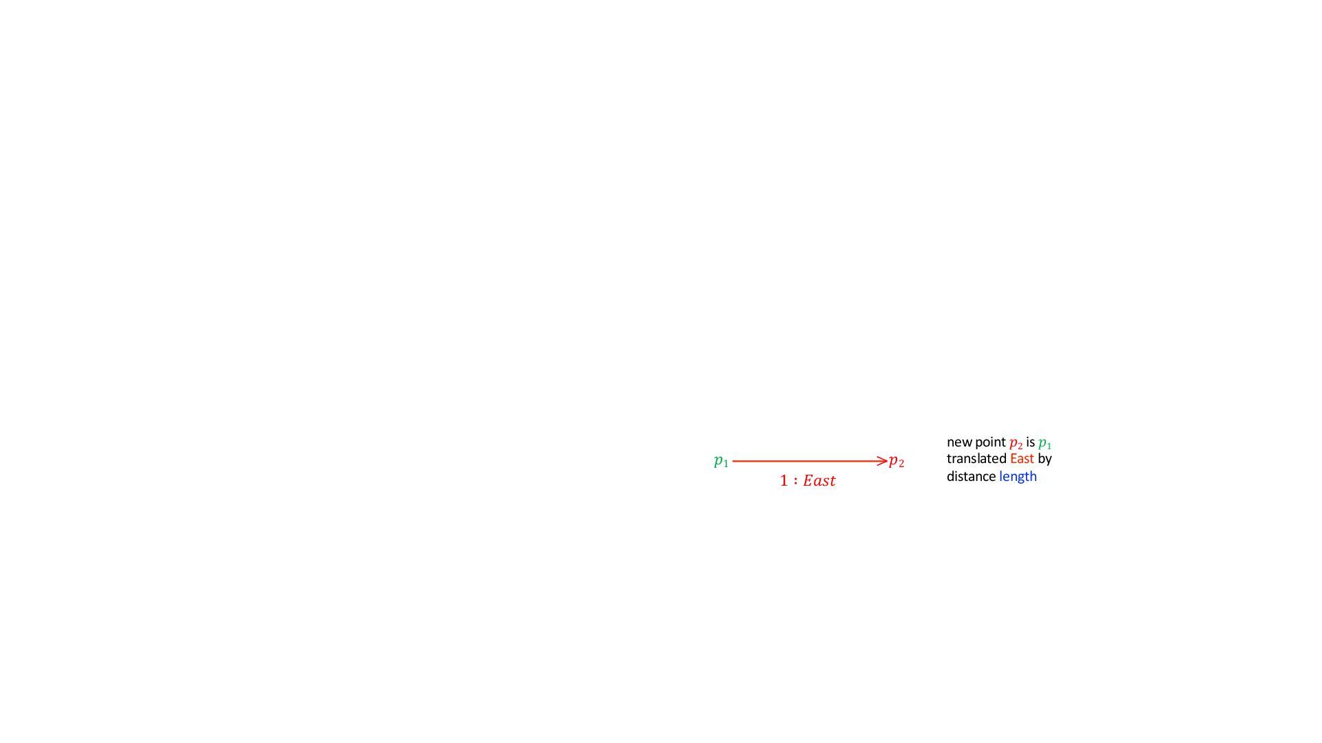
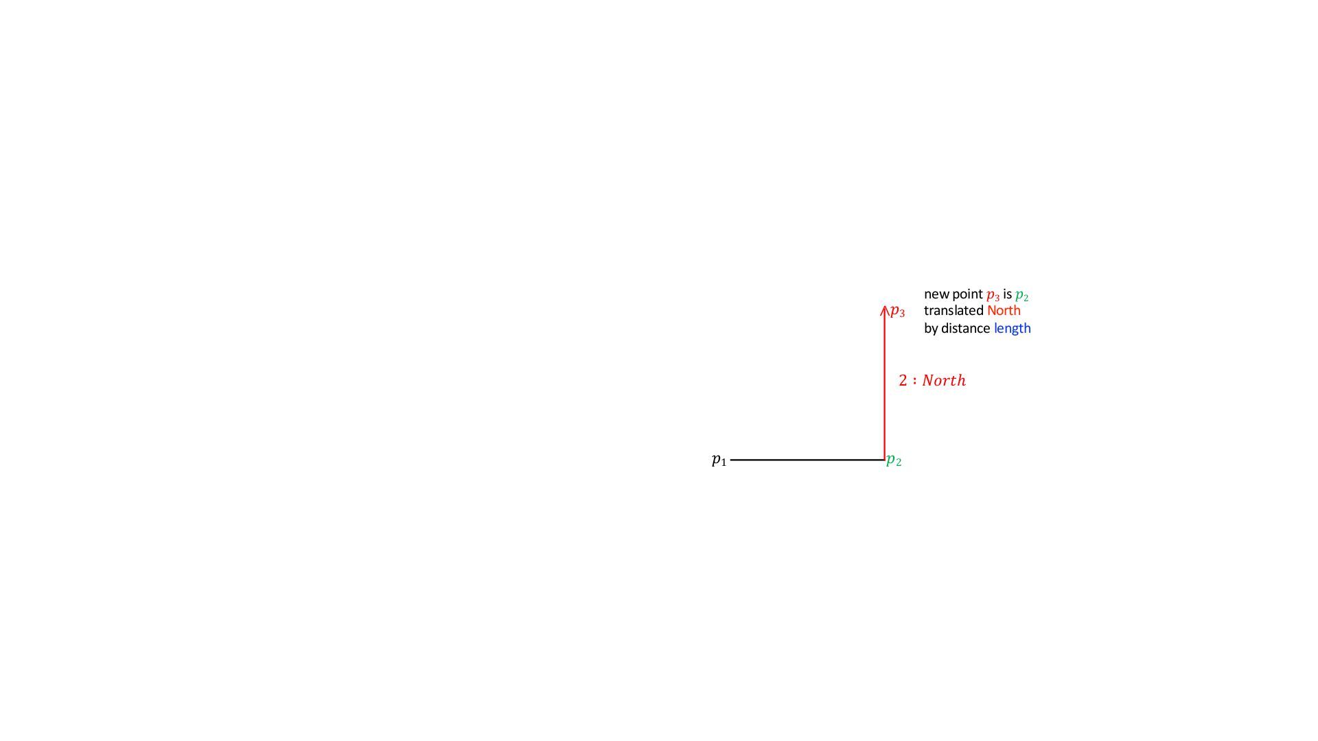
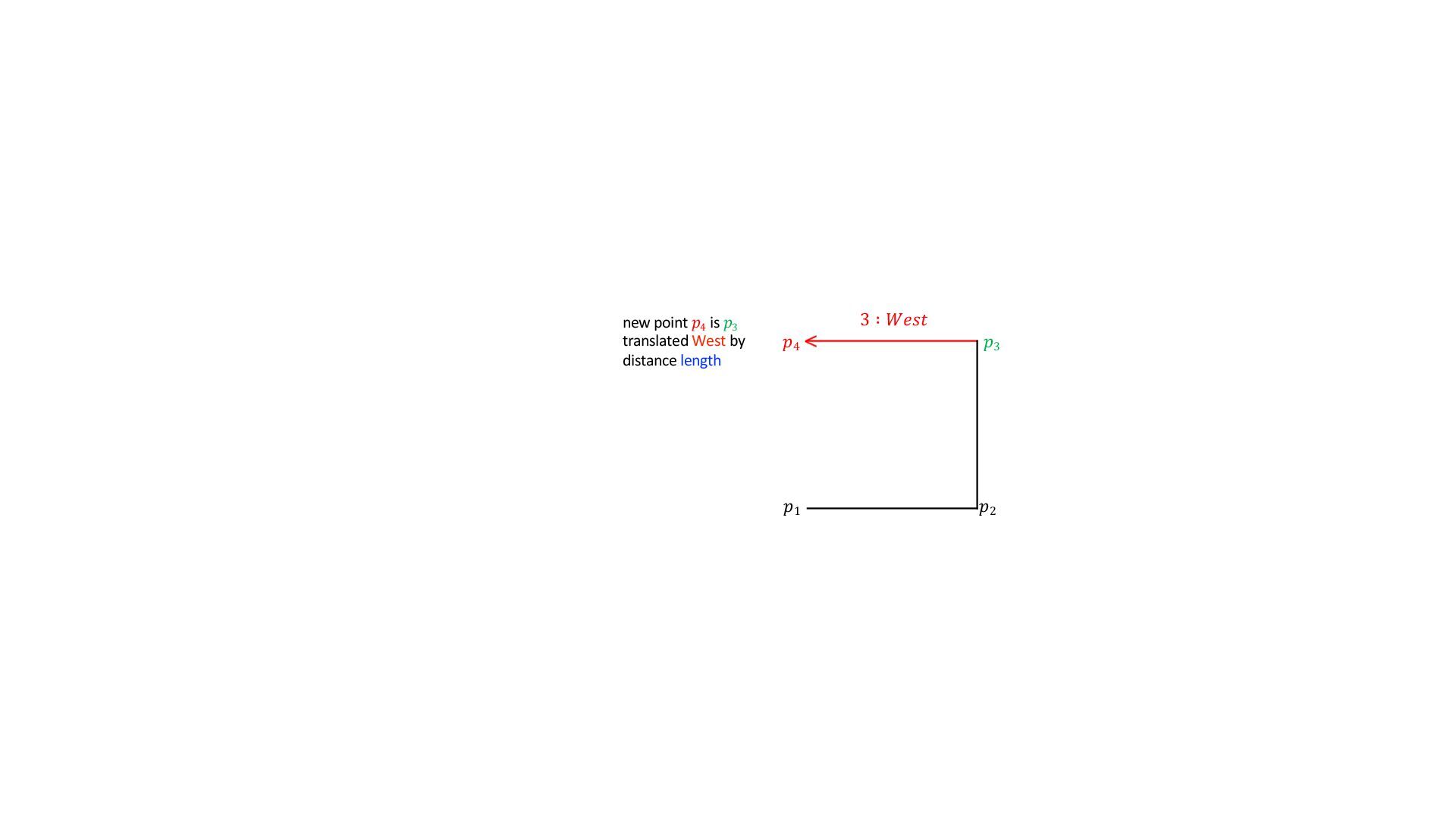
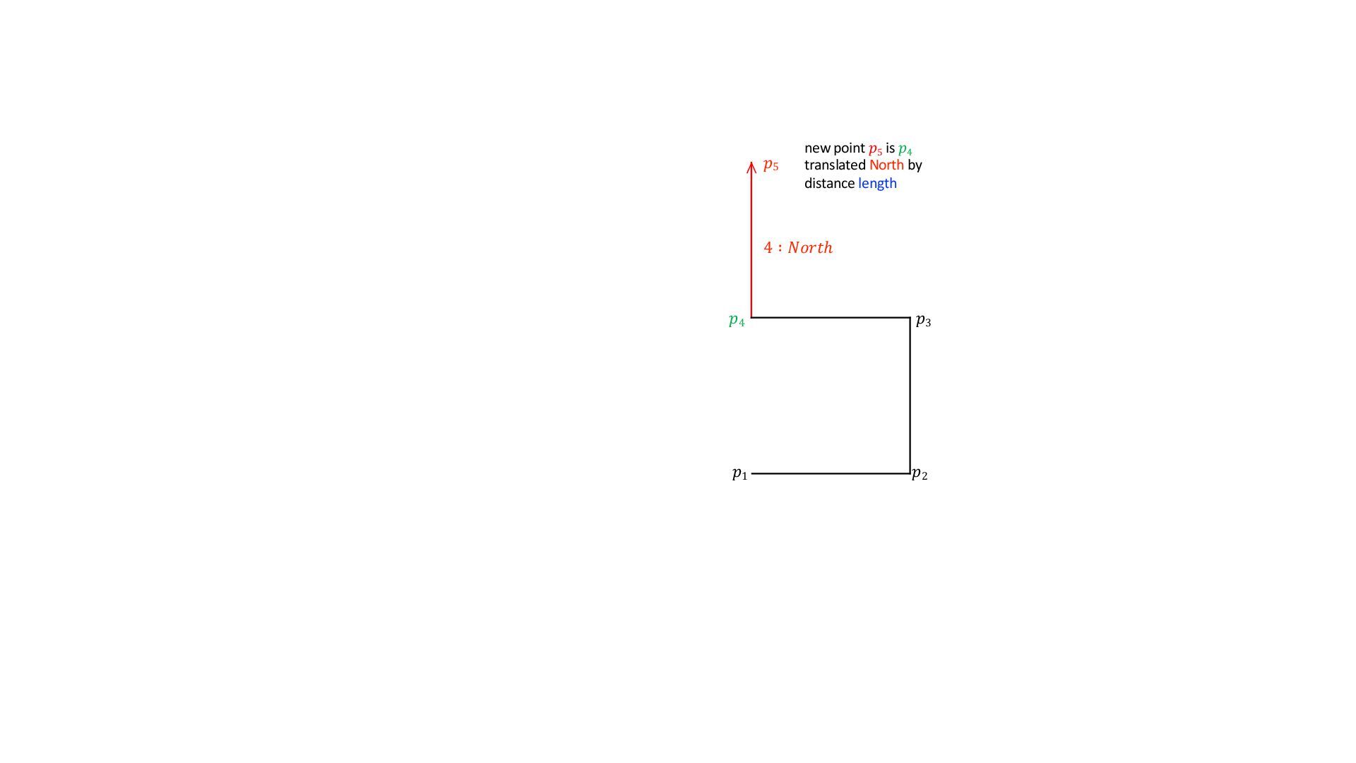
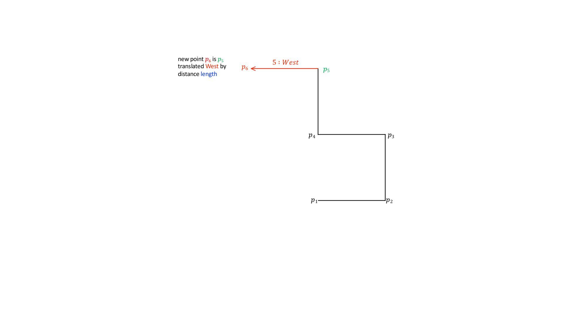
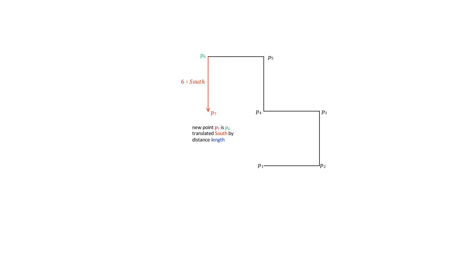
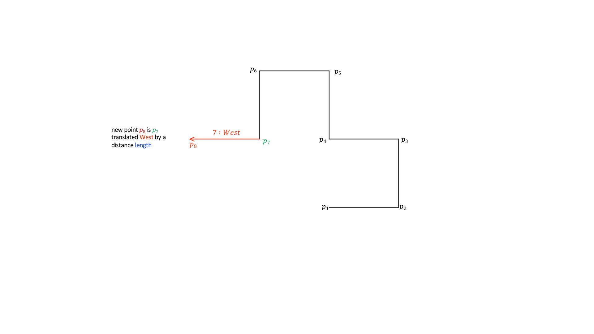
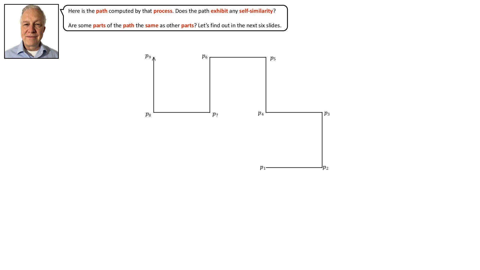
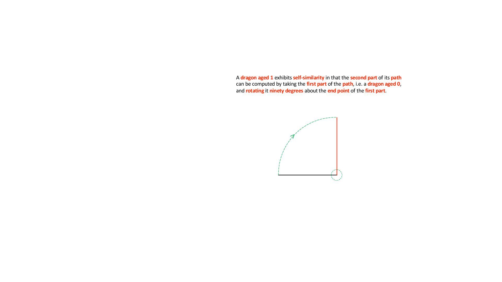
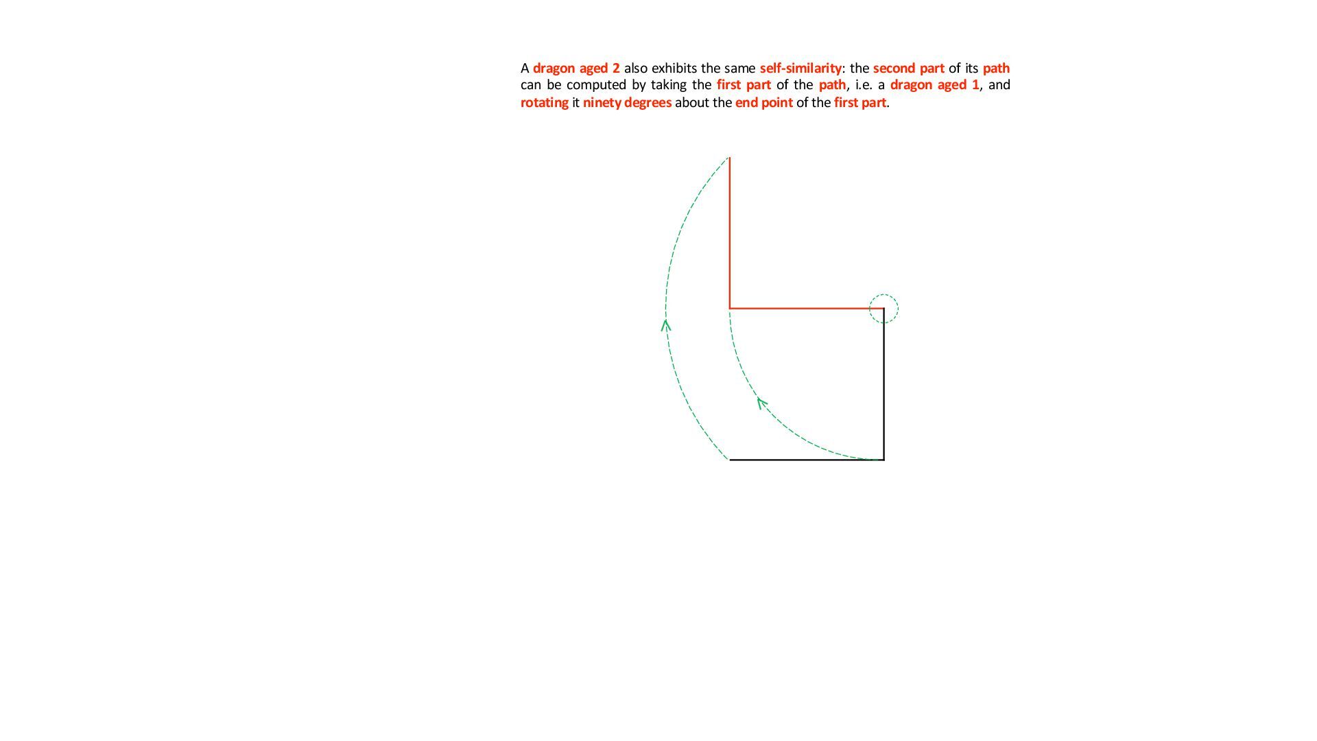
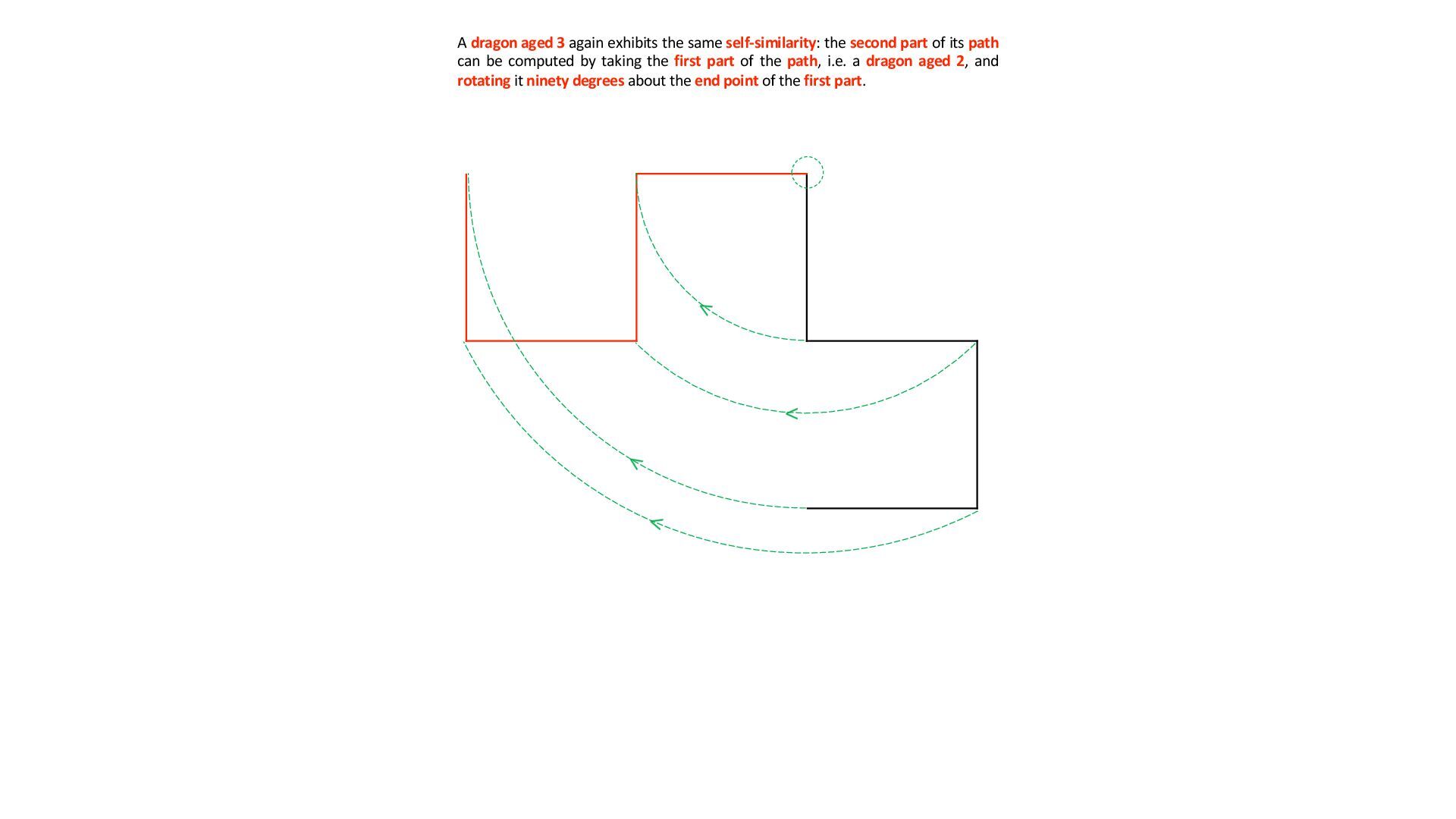
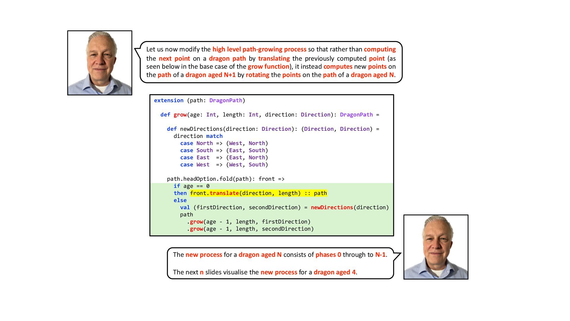
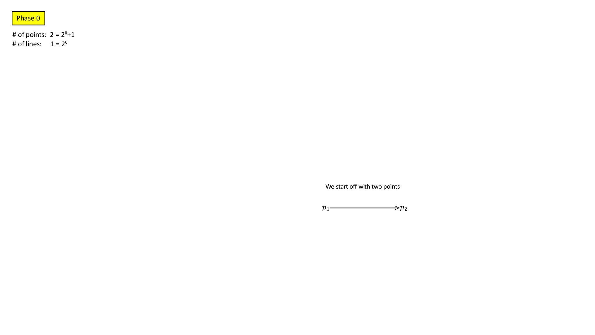
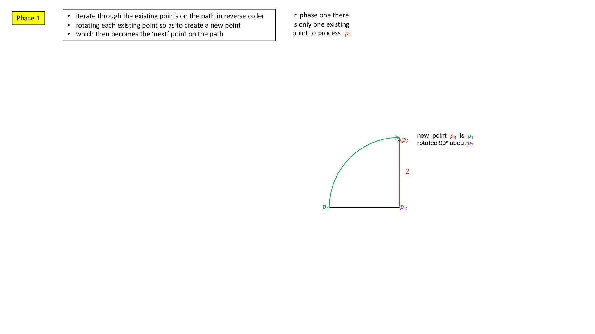
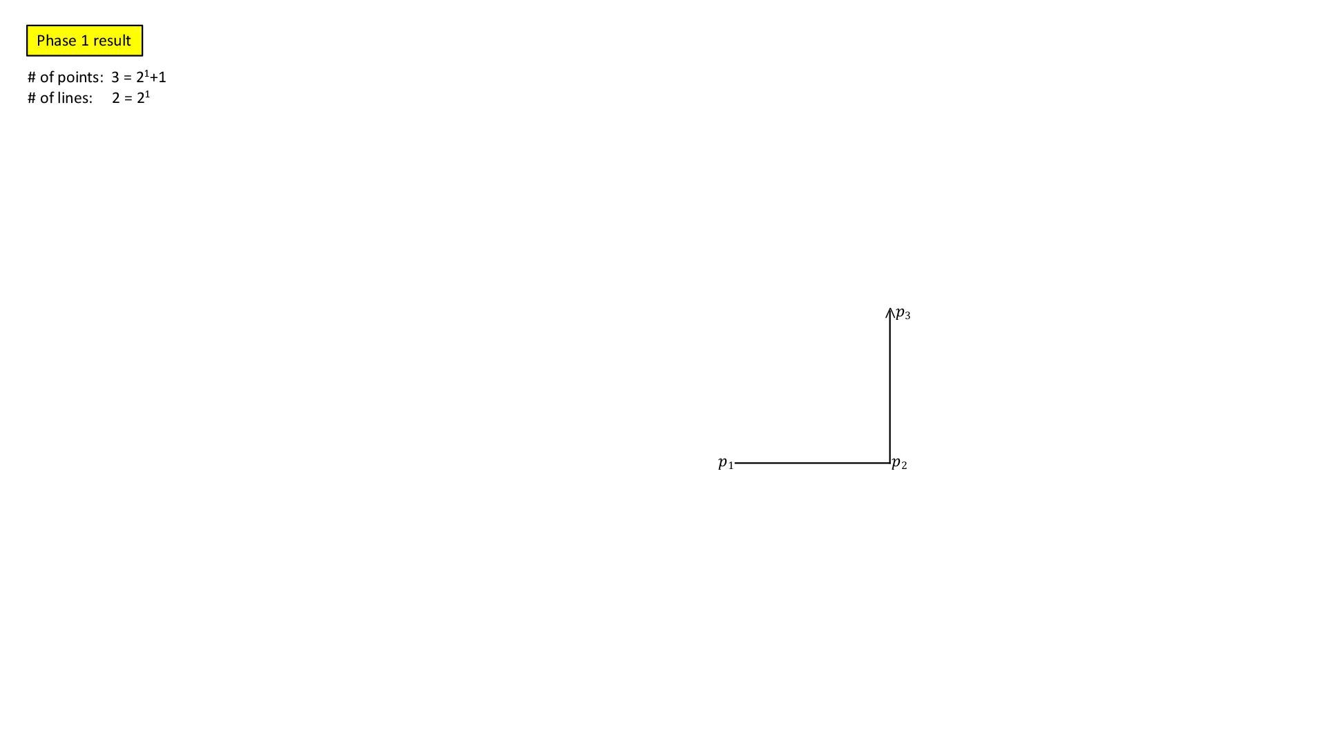
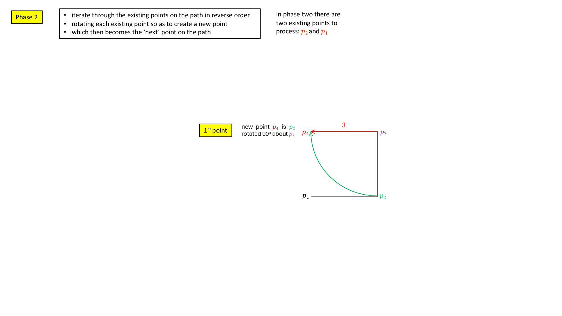
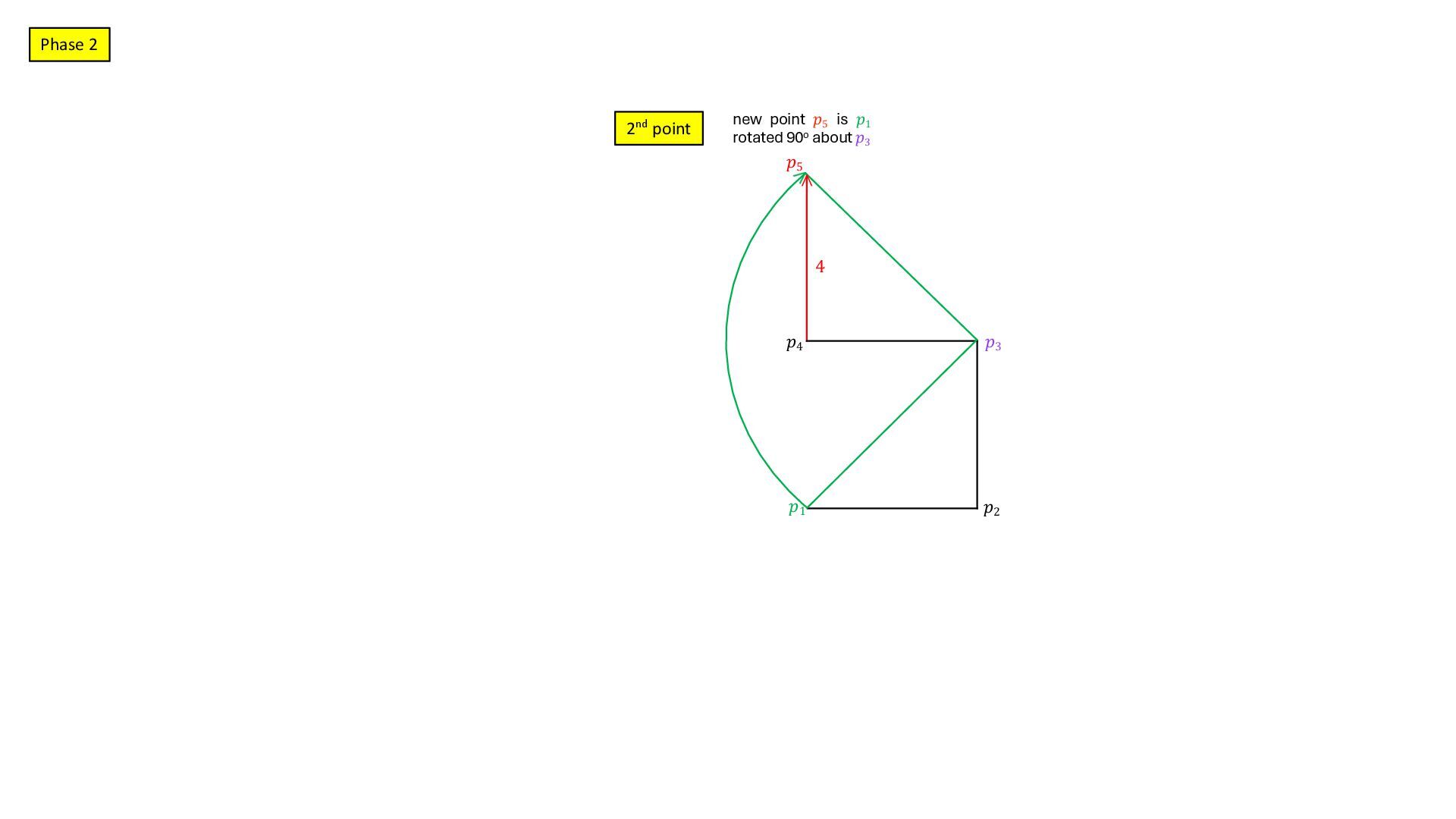
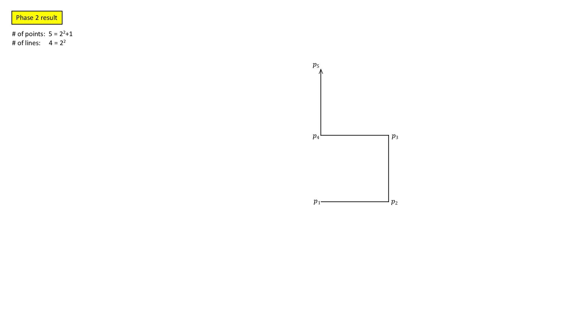
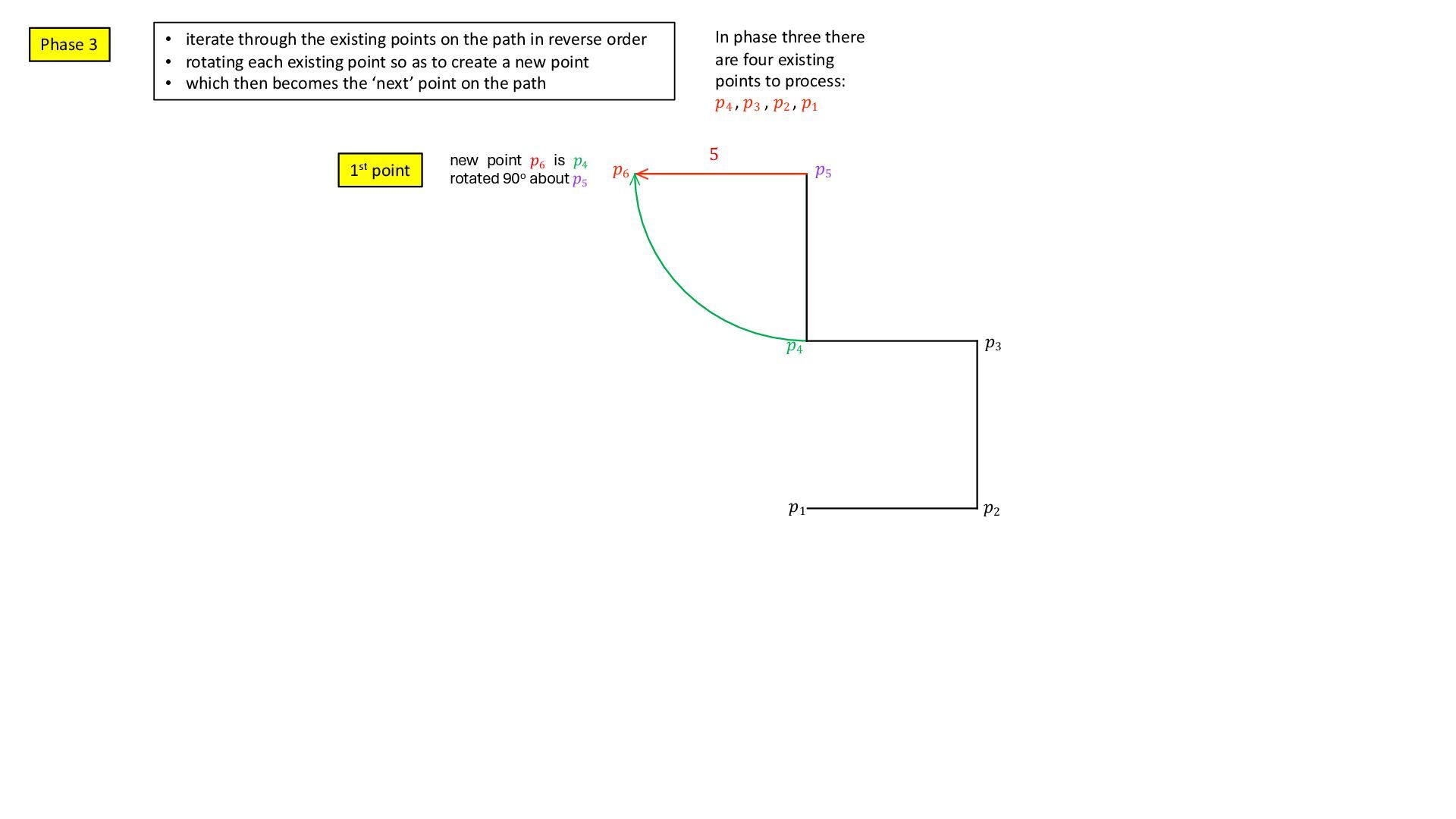
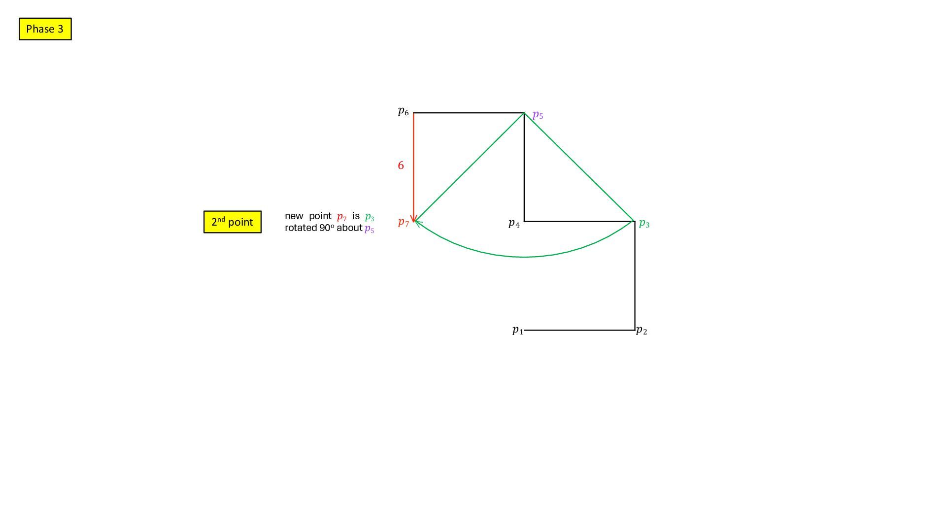
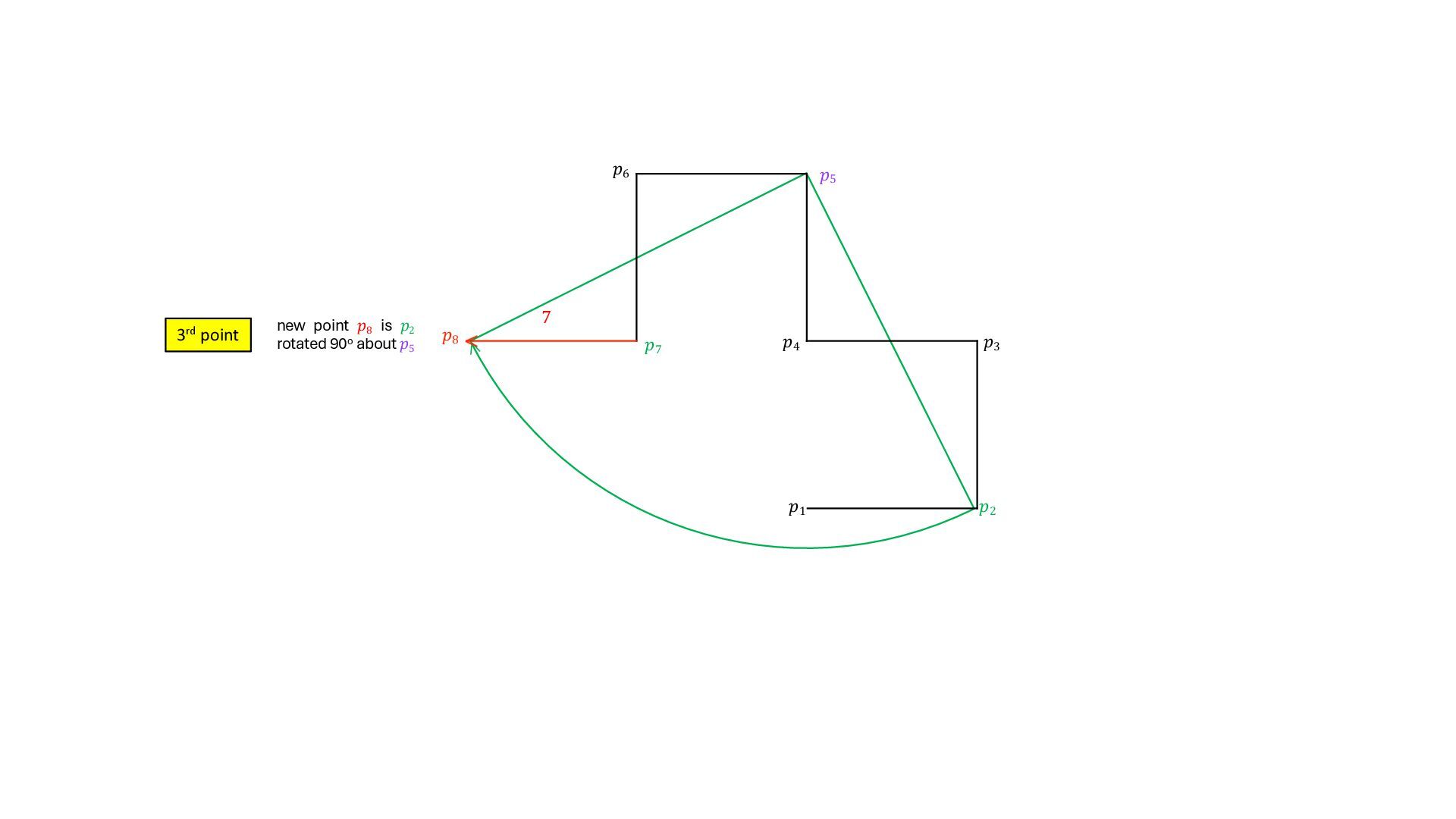
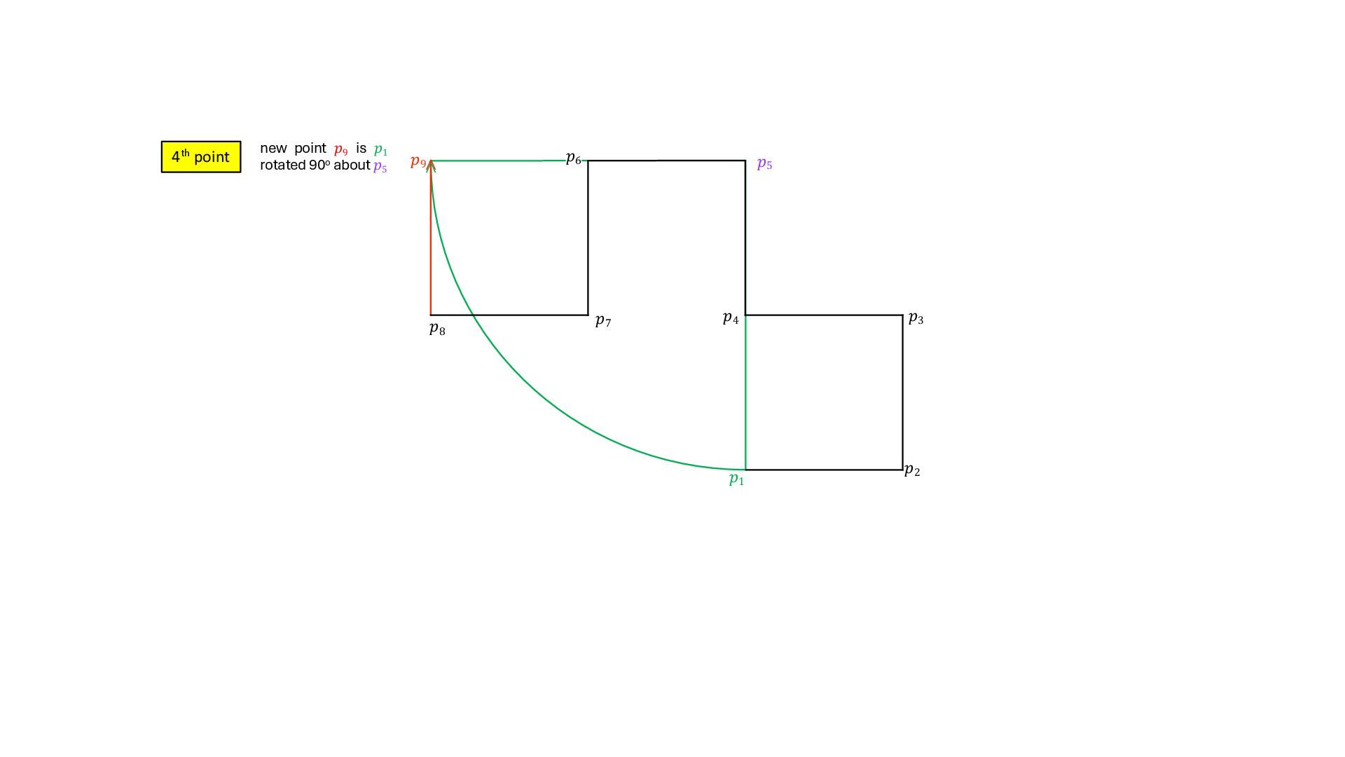
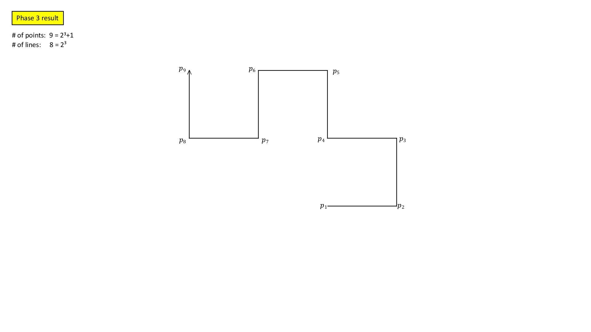
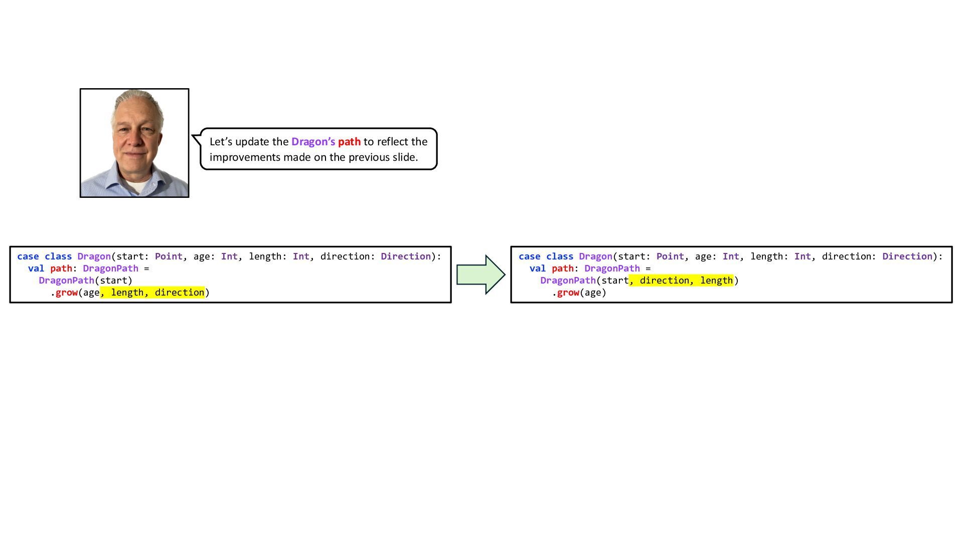
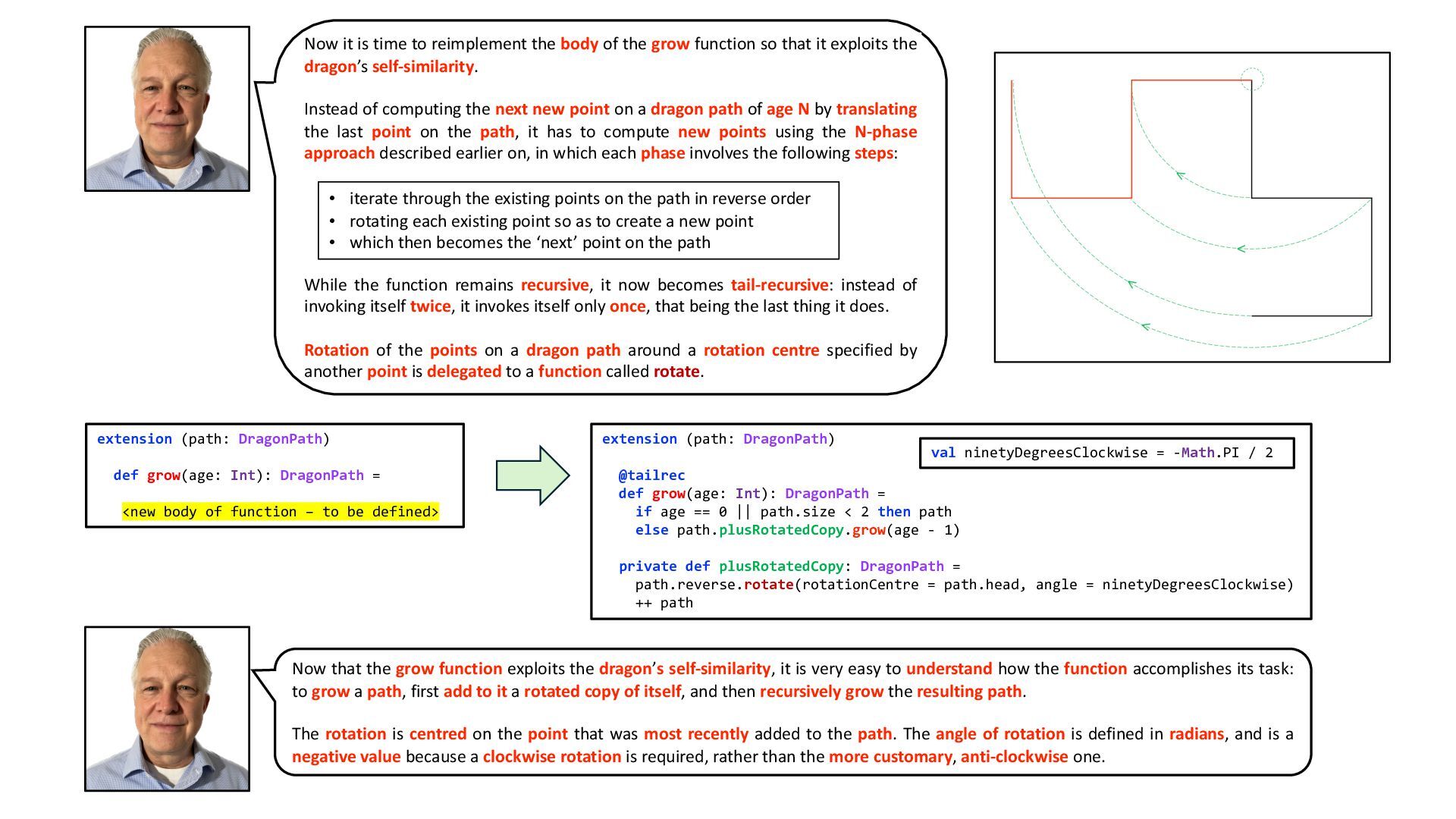
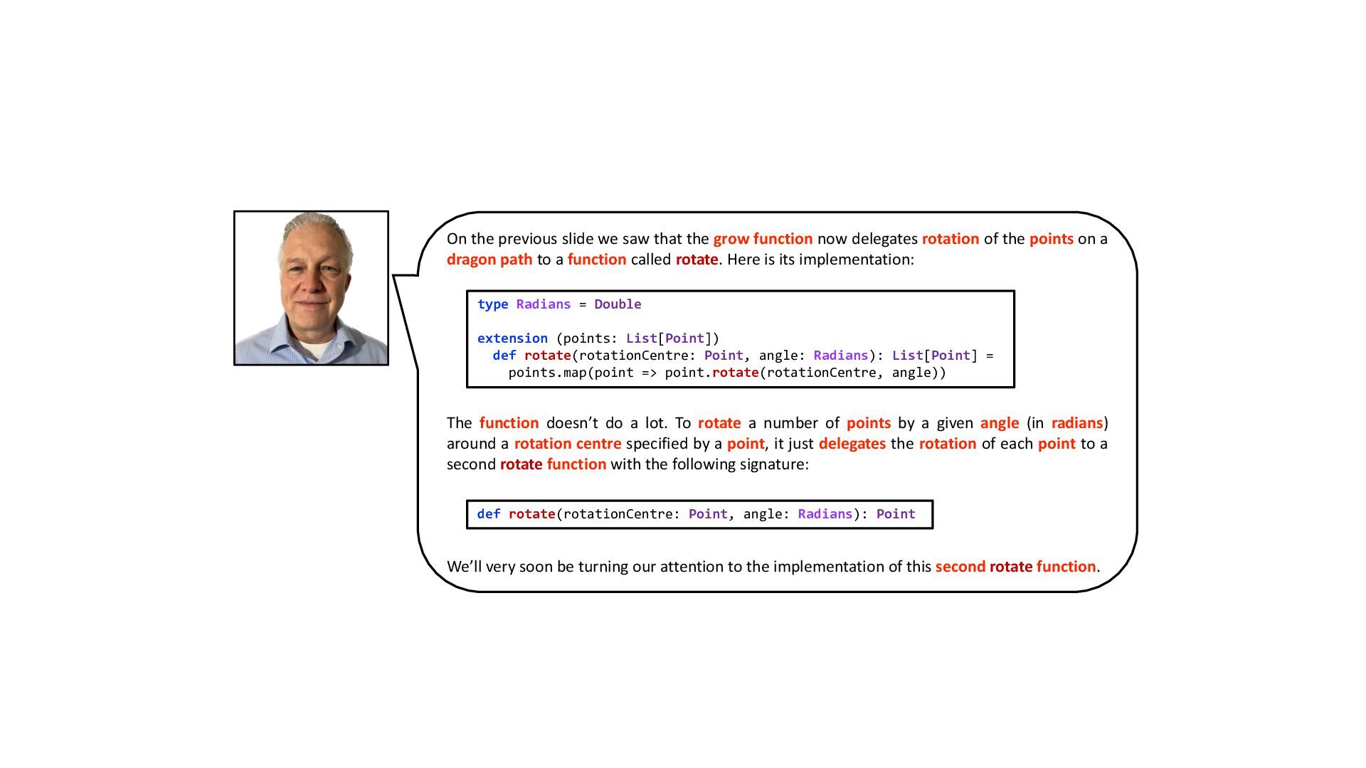
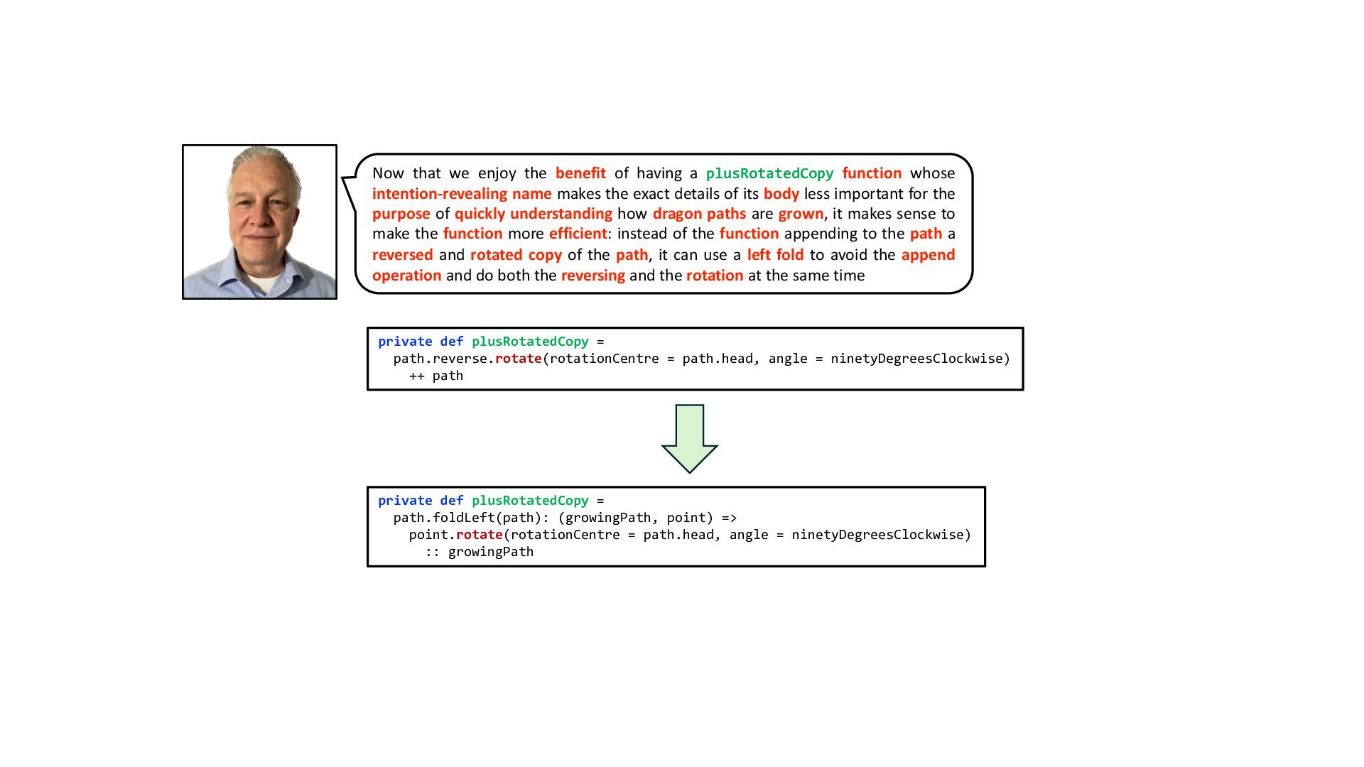
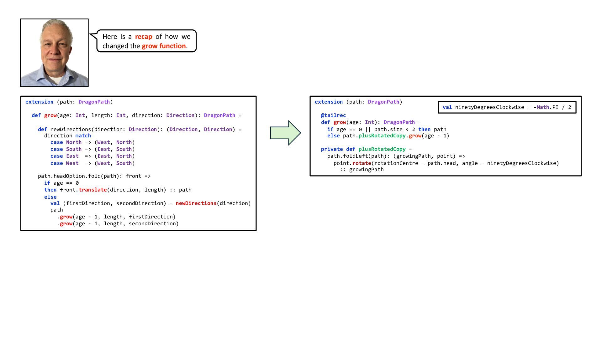
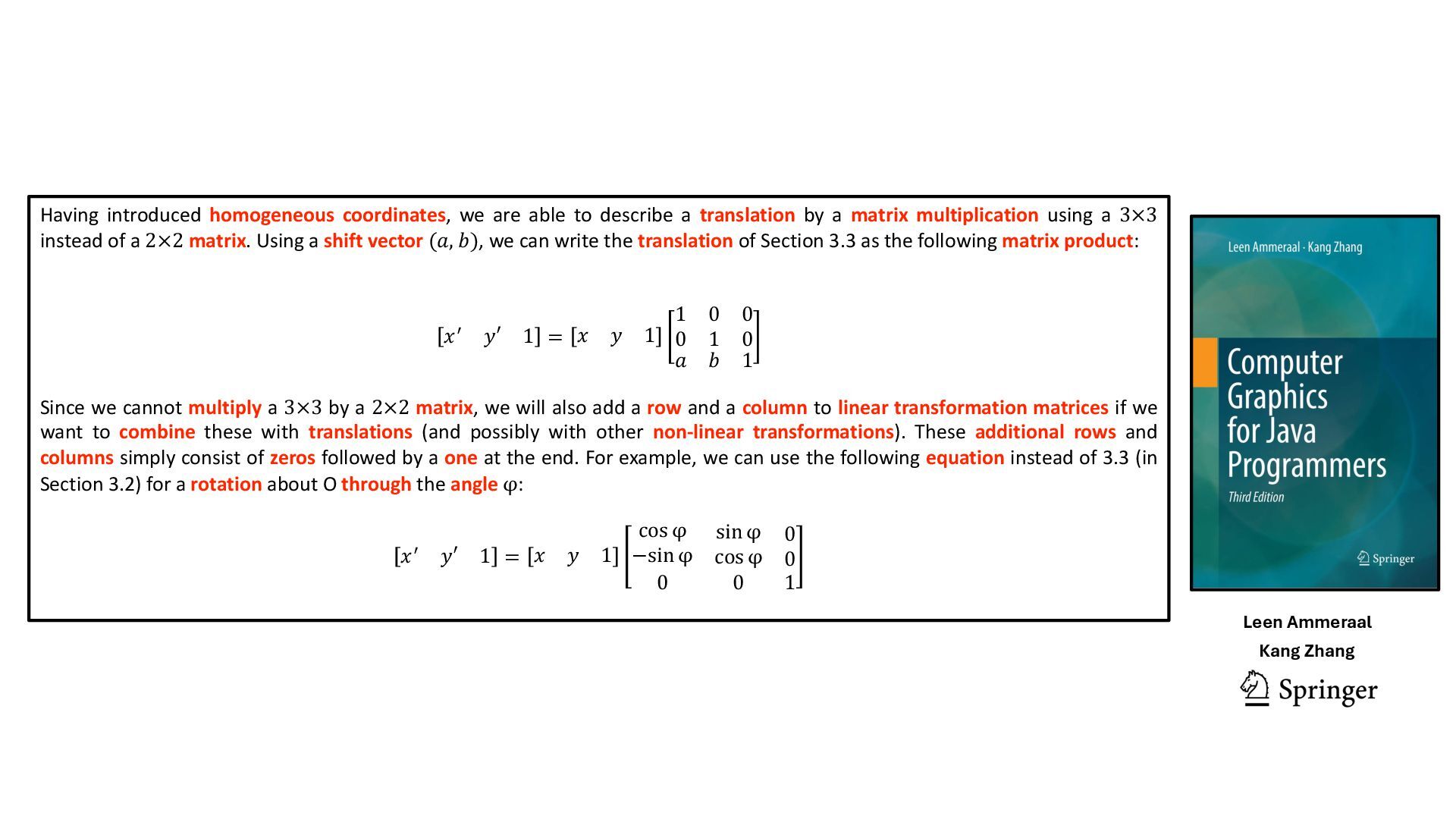
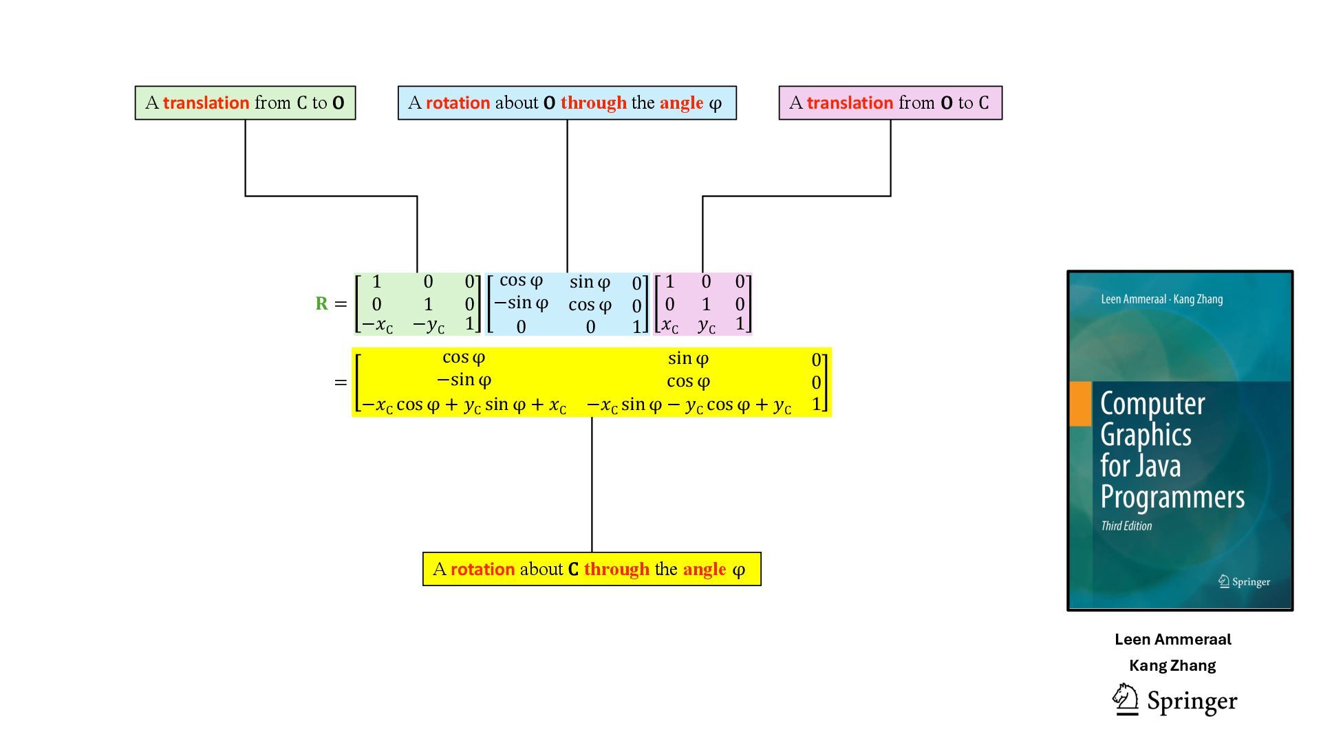
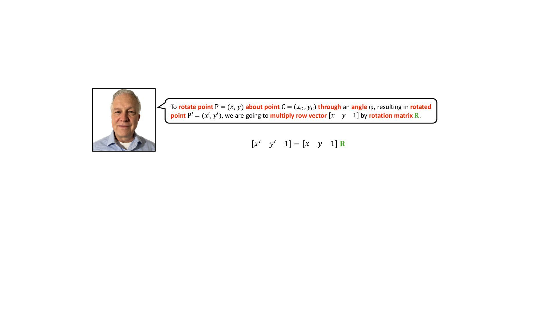
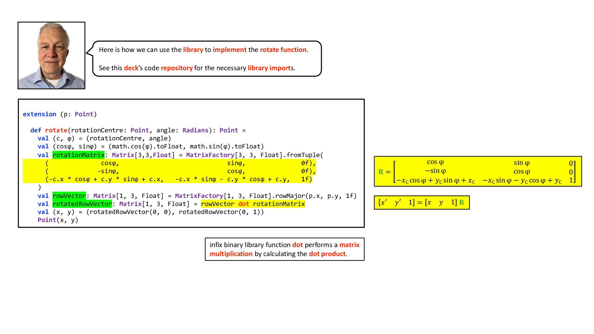
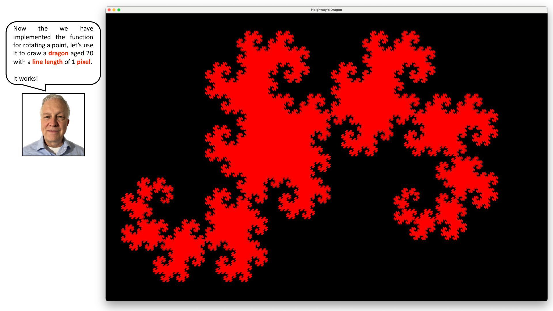
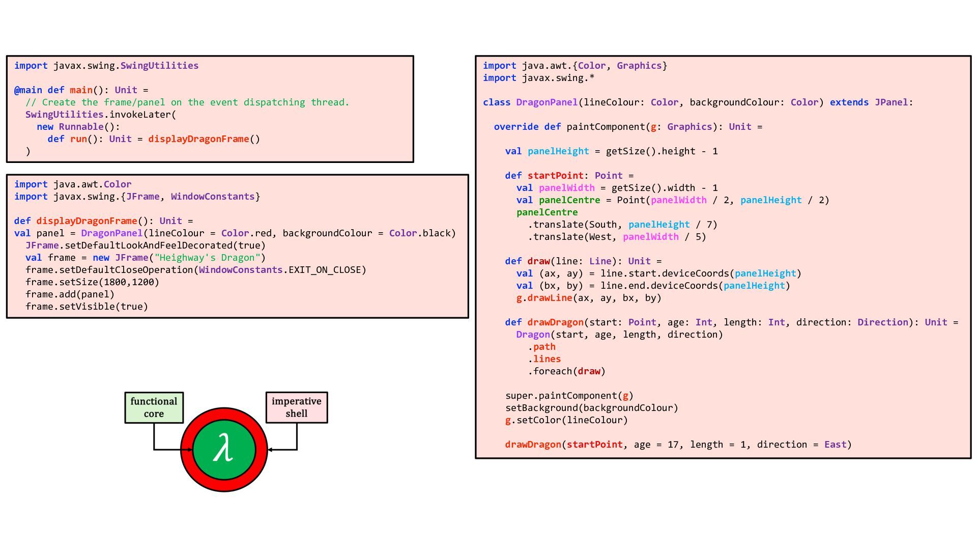
61. type DragonPath = List[Point] val ninetyDegreesClockwise: Radians = -Math.PI / 2 object DragonPath: def apply(startPoint : Point, direction: Direction, length: Int): DragonPath = val nextPoint = startPoint.translate(direction, amount = length) List(nextPoint, startPoint) extension (path: DragonPath) def lines: List[Line] = if path.length < 2 then Nil else path.zip(path.tail) @tailrec def grow(age: Int): DragonPath = if age == 0 || path.size < 2 then path else path.plusRotatedCopy.grow(age - 1) private def plusRotatedCopy = path.reverse.rotate(rotationCentre=path.head, angle=ninetyDegreesClockwise) ++ path case class Dragon(start: Point, age: Int, length: Int, direction: Direction): val path: DragonPath = DragonPath(start, direction, length) .grow(age) case class Point(x: Float, y: Float) type Radians = Double extension (p: Point) def deviceCoords(panelHeight: Int): (Int, Int) = (Math.round(p.x), panelHeight - Math.round(p.y)) def translate(direction: Direction, amount: Float): Point = direction match case North => Point(p.x, p.y + amount) case South => Point(p.x, p.y - amount) case East => Point(p.x + amount, p.y) case West => Point(p.x - amount, p.y) def rotate(rotationCentre: Point, angle: Radians): Point = val (c, ϕ) = (rotationCentre, angle) val (cosϕ, sinϕ) = (math.cos(ϕ).toFloat, math.sin(ϕ).toFloat) val rotationMatrix: Matrix[3,3,Float] = MatrixFactory[3, 3, Float].fromTuple( ( cosϕ, sinϕ, 0f), ( -sinϕ, cosϕ, 0f), (-c.x * cosϕ + c.y * sinϕ + c.x, -c.x * sinϕ - c.y * cosϕ + c.y, 1f) ) val rowVector: Matrix[1,3,Float] = MatrixFactory[1,3,Float].rowMajor(p.x,p.y,1f) val rotatedRowVector: Matrix[1, 3, Float] = rowVector dot rotationMatrix val (x, y) = (rotatedRowVector(0, 0), rotatedRowVector(0, 1)) Point(x, y) extension (points: List[Point]) def rotate(rotationCentre: Point, angle: Radians) : List[Point] = points.map(point => point.rotate(rotationCentre, angle)) type Line = (Point, Point) extension (line: Line) def start: Point = line(0) def end: Point = line(1) enum Direction: case North, East, South, West
62. I hope you enjoyed that. See you in part three.