Accelerated Stein Variational Gradient Flow

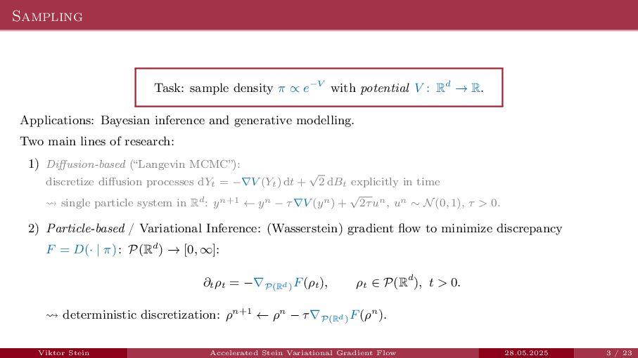
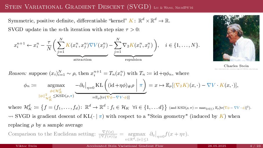
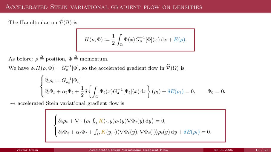
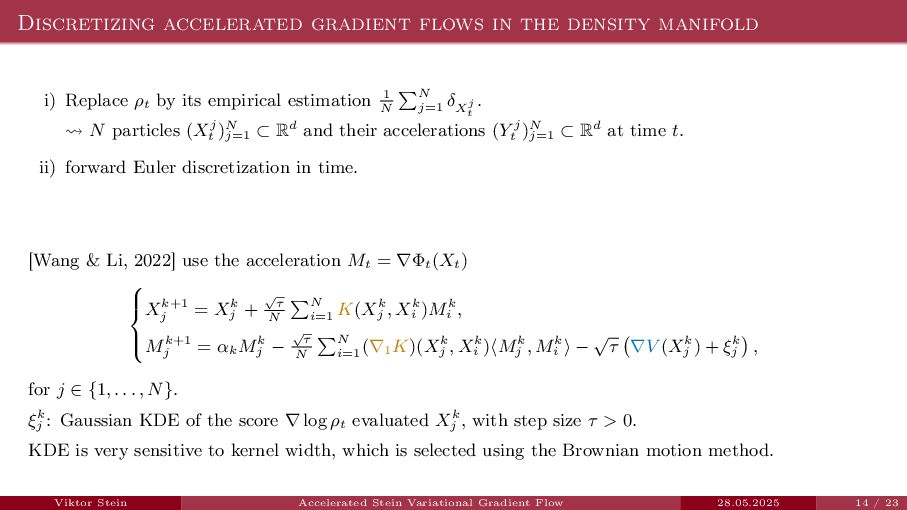
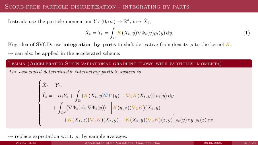
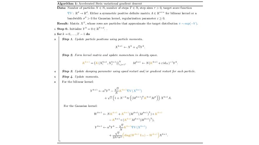
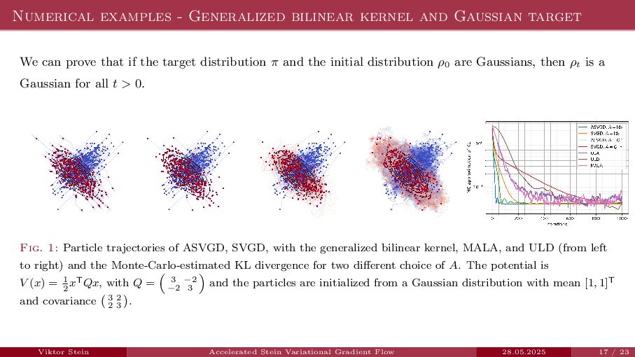
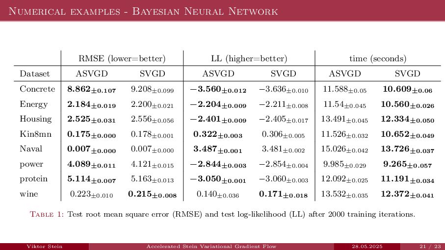
Stein variational gradient descent (SVGD) is a kernel-based particle method for sampling from a target distribution, e.g., in generative modeling and Bayesian inference. SVGD does not require estimating the gradient of the log-density, which is called score estimation. In practice, SVGD can be slow compared to score-estimation based sampling algorithms. To design fast and efficient high-dimensional sampling algorithms, we introduce ASVGD, an accelerated SVGD, based on an accelerated gradient flow in a metric space of probability densities following Nesterov's method. We then derive a momentum-based discrete-time sampling algorithm, which evolves a set of particles deterministically. To stabilize the particles' momentum update, we also study a Wasserstein metric regularization. For the generalized bilinear kernel and the Gaussian kernel, toy numerical examples with varied target distributions demonstrate the effectiveness of ASVGD compared to SVGD and other popular sampling methods.
This is joint work with Wuchen Li (University of South Carolina)

Preprint: https://arxiv.org/abs/2503.23462
Code: https://github.com/ViktorAJStein/Accelerated_Stein_Variational_Gradient_Flows/tree/main

Transcript

1. Accelerated Stein Variational Gradient Flow joint work with Wuchen Li, University of South Carolina UCLA level set seminar (Stan Osher). Viktor Stein (TU Berlin), 21.04.2025
2. 1. Sampling from densities 2. Stein Variational Gradient Descent 3. Nesterov’s accelerated gradient descent 4. (Accelerated) Stein Gradient Flow in the density manifold 5. Particle discretization 6. Numerical examples
3. Sampling Task: sample density π ∝ e−V with potential V : Rd → R. Applications: Bayesian inference and generative modelling. Two main lines of research: • Diffusion-based (“Langevin MCMC”): discretize diffusion processes dYt = −∇V (Yt) dt + √ 2 dBt explicitly in time ⇝ single particle system in Rd: yn+1 ← yn − τ∇V (yn) + √ 2un+1, un+1 ∼ N(0, 1), τ > 0. • Particle-based / Variational Inference: (Wasserstein) gradient flow to minimize discrepancy F = D(· | π): ∂t ρt = −∇F(ρt ), ρt ∈ P(Rd), t > 0. ⇝ deterministic discretization: ρn+1 ← ρn − τ∇F(ρn). Viktor Stein Accelerated Stein Variational Gradient Flow 21.04.2025 3 / 21
4. Stein Variational Gradient Descent Liu and Wang, 2016 Symmetric, positive definite, differentiable “kernel” K : Rd × Rd → R. SVGD update: xn+1 i ← xn i − τ N N j=1 K(xn i , xn j )∇V (xn j ) attraction − N j=1 ∇2 K(xn i , xn j ) repulsion , i ∈ {1, . . . , N}. Charles Stein https://news.stanford.edu/__data/assets/image/0027/70758/Obit_stein_feach.jpeg Reason: suppose (xi)N i=1 ∼ ρ, then xi+1 = Ti (xi ) with Ti := id +ηϕi , where ϕi = argmax ϕ∈HK ∥ϕ∥HK ≤1 −∂η η=0 KL ((Ti )# ρ | π) = argmax ϕ∈HK ∥ϕ∥HK ≤1 Eρ [∇V · ϕ + ∇ϕ]. ⇝ SVGD is gradient descent of KL(· | π) with respect to a "Stein geometry" (induced by K) when replacing ρ by a sample average Comparison to the Euclidean setting: ∇f(x) ∥∇f(x)∥2 = argmax v∈R d ∥v∥≤1 ∂t t=0 f(x + tv). Viktor Stein Accelerated Stein Variational Gradient Flow 21.04.2025 4 / 21
5. Which kernel to choose? smoothness radial not radial Gauss exp − 1 2σ2 ∥x − y∥2 2 Bilinear xTAy + 1 Laplace exp (−∥x − y∥2 ) Inverse multiquadric (∥x − y∥2 2 + s)− 1 2 Mat´ ern Riesz, s ∈ (0, 1) ∥x∥2s 2 + ∥y∥2s 2 − ∥x − y∥2s 2 Viktor Stein Accelerated Stein Variational Gradient Flow 21.04.2025 5 / 21
6. Accelerating gradient descent Goal: find minimizer x∗ of convex, differentiable function f : Rd → R with L-Lipschitz gradient. Gradient descent with step size τ ∈ 0, 2 L xn+1 ← xn − τ∇f(xn), n ∈ N converges linearly: f(xn) − f(x∗) ∈ O(n−1). Nesterov’s accelerated gradient descent:      xn+1 = yn − τ∇f(yn) gradient step yn+1 = xn+1 + αn+1 (xn+1 − xn) momentum step converges quadratically: f(xn) − f(x∗) ∈ O(n−2). Damping: αn = n−1 n+2 or αn = √ L− √ β √ L+ √ β if f is β-strongly convex. Yurii Nesterov https://upload.wikimedia.org/wikipedia/commons/9/9e/Nesterov_yurii.jpg Viktor Stein Accelerated Stein Variational Gradient Flow 21.04.2025 6 / 21
7. Animation: accelerated gradient descent https://distill.pub/2017/momentum/ [Goh17, OC15, SBC16] Viktor Stein Accelerated Stein Variational Gradient Flow 21.04.2025 7 / 21
8. Improving Nesterov’s method in practice: restart techniques Gradient descent: monotone decreasing functional values Accelerated methods: “ripples”. momentum too high: trajectory overshoots the minimum, os- cillates around it. momentum too low: not enough exploration, slow convergence. ⇝ restart momentum = set αk ← 0, when • Function restart: f(xk ) > f(xk−1 ) (not feasible for sampling) • Gradient restart: ⟨∇f(xk ), xk − xk−1 ⟩ < 0. • Speed restart: ∥xk+1 − xk ∥ < ∥xk − xk−1 ∥. Gradient descent, accelerated, accelerated + adaptive restart. O’Donoghue, Candés: Adaptive Restart for Accelerated Gradient Schemes (Found Comput Math 15 2015). Su, Boyd, Candés: A Differential Equation for Modeling Nesterov’s Accelerated Gradient Method: Theory and Insights. JMLR 17 (2016) Viktor Stein Accelerated Stein Variational Gradient Flow 21.04.2025 8 / 21
9. The density manifold The set of smooth positive probability densities P(Ω) := ρ ∈ C∞(Ω) : ρ(x) > 0 ∀x ∈ Ω, Ω ρ(x) dx = 1 . with its Fréchet topology, forms an infinite-dimensional C∞-Fréchet manifold, if Ω is compact Riemannian manifold w/o boundary equipped with its volume measure. • (Kinematic) tangent space to P(Ω) at ρ: Tρ P(Ω) := σ ∈ C∞(Ω) : Ω σ(x) dx = 0 . • Cotangent space T∗ ρ P(Ω) := C∞(Ω)/ R. (Note: Tρ P(Ω)∗ ̸= T∗ ρ P(Ω).) • Metric tensor field on P(Ω) = smooth map G: P(Ω) ∋ ρ → Gρ such that ∀ρ ∈ P(Ω), Gρ : Tρ P(Ω) → T∗ ρ P(Ω) is smooth & invertible. John Lafferty https://wti.yale.edu/profile/john-lafferty Viktor Stein Accelerated Stein Variational Gradient Flow 21.04.2025 9 / 21
10. Gradient flows in the density manifold Definition (First linear functional derivative) If it exists, the first functional derivative of E : P(Ω) → R is δE : P(Ω) → C∞(Ω)/ R with ⟨δE(ρ), ϕ⟩L2(Ω) = ∂t t=0 E(ρ + tϕ), ∀ϕ ∈ C∞(Ω) : ρ + tϕ ∈ P(Ω), |t| small. Definition (Metric gradient flow on P(Ω)) A smooth curve ρ: [0, ∞) → P(Ω), t → ρt is a (P(Ω), G)-gradient flow of E starting at ρ(0) if ∂t ρt = −G−1 ρt [δE(ρt )], ∀t > 0. Intuition: inverse metric tensor deforms linear derivative δE. Viktor Stein Accelerated Stein Variational Gradient Flow 21.04.2025 10 / 21
11. Wasserstein and Stein variational gradient flow on densities The Wasserstein metric defined via [GW ρ ]−1[Φ] := −∇ · (ρ∇Φ), ρ ∈ P(Ω). The (P(Ω), GW )-gradient flow of E = KL(· | Z−1e−V ) is ∂tρt = ∇ · (ρt(∇ log ρt + ∇V )) = ∆ρt + ∇ · (ρt∇V ), where we used ρt∇ log ρt = ∇ρt. Stein metric defined via: (G(K) ρ )−1(Φ) := x → −∇x · ρ(x) Ω K(x, y)ρ(y)∇Φ(y) dy . The (P(Ω), GK )-gradient flow of E = KL(· | Z−1e−V ) is ∂t ρt (x) = ∇x · ρt (x) Ω K(x, y)ρt (y)(∇ log ρt (y) + ∇V (y)) dy = ∇x · ρt (x) Ω (K(x, y)∇V (y) − ∇2 K(x, y)) ρt (y) dy . (we used ρt ∇ log ρt = ∇ρt and applied integration by parts to the score function ∇ log ρt ) Viktor Stein Accelerated Stein Variational Gradient Flow 21.04.2025 11 / 21
12. Accelerated gradient flows: from Rd to P(Ω) The continuous time limit of accelerated gradient descent is the 2nd order ODE ¨ xt + αt ˙ xt + ∇f(xt ) = 0, where αt = 3 t or αt = 2 √ β. This can be rewritten as damped Hamiltonian flow:   ˙ xt ˙ pt   +   0 αt pt   −   0 id − id 0     ∇x H(xt , pt ) ∇p H(xt , pt ),   = 0. Emmanuel Candés https://stanforddaily.com/2017/11/07/qa-with-new-macarthur-fellow-emmanuel-candes/ where x ∈ Rd represents position, p = ˙ x ∈ Rd represents momentum, and the Hamiltonian is H(x, p) := 1 2 ∥p∥2 2 + f(x) = kinetic energy + potential energy ⇝ this formulation can be generalized from Rd to P(Ω). Viktor Stein Accelerated Stein Variational Gradient Flow 21.04.2025 12 / 21
13. Accelerated Stein variational gradient flow on densities The Hamiltonian on P(Ω) is H(ρ, Φ) := 1 2 Ω Φ(x)G−1 ρ [Φ](x) dx + E(ρ). As before: ρ ∆ = position, Φ ∆ = momentum. We have δ2 H(ρ, Φ) = G−1 ρ [Φ], so the accelerated gradient flow in P(Ω) is      ∂t ρt = G−1 ρt [Φt ] ∂t Φt + αt Φt + 1 2 δ Ω Φt (x)G−1 • [Φt ](x) dx (ρt ) + δE(ρt ) = 0, Φ0 = 0. ⇝ accelerated Stein variational gradient flow is      ∂t ρt + ∇ · ρt Ω K(·, y)ρt (y)∇Φt (y) dy = 0, ∂t Φt + αt Φt + Ω K(y, ·)⟨∇Φt (y), ∇Φt (·)⟩ρt (y) dy + δE(ρt ) = 0. Viktor Stein Accelerated Stein Variational Gradient Flow 21.04.2025 13 / 21
14. Discretizing accelerated gradient flows in the density manifold i) Replace ρt by its empirical estimation 1 N N j=1 δ Xj t . ⇝ N particles (Xj t )N j=1 ⊂ Rd and their accelerations (Y j t )N j=1 ⊂ Rd at time t. ii) forward Euler discretization in time. [Wang & Li, 2022] use the acceleration Mt = ∇Φt (Xt )      Xk+1 j = Xk j + √ τ N N i=1 K(Xk j , Xk i )Mk i , Mk+1 j = αk Mk j − √ τ N N i=1 (∇1 K)(Xk j , Xk i )⟨Mk j , Mk i ⟩ − √ τ ∇V (Xk j ) + ξk j , for j ∈ {1, . . . , N}. ξk j : Gaussian KDE of the score ∇ log ρt evaluated Xk j , with step size τ > 0. KDE is very sensitive to kernel width, which is selected using the Brownian motion method. Viktor Stein Accelerated Stein Variational Gradient Flow 21.04.2025 14 / 21
15. Score-free particle discretization - integrating by parts Instead: use the particle momentum Y : (0, ∞) → Rd, t → ˙ Xt , ˙ Xt = Yt = Ω K(Xt , y)∇Φt (y)ρt (y) dy. (1) Key idea of SVGD: use integration by parts to shift derivative from density ρ to the kernel K. ⇝ can also be applied in the accelerated scheme: Lemma (Accelerated Stein variational gradient flows with particles’ momenta) The associated deterministic interacting particle system is                      ˙ Xt = Yt , ˙ Yt = −αt Yt + Ω (K(Xt , y)∇V (y) − ∇2 K(Xt , y)) ρt (y) dy + Ω2 ⟨∇Φt (z), ∇Φt (y)⟩ · K(y, z)(∇2 K)(Xt , y) +K(Xt , z)(∇1 K)(Xt , y) − K(Xt , y)(∇2 K)(z, y) ρt (y) dy ρt (z) dz. ⇝ replace expectation w.r.t. ρt by sample averages. Viktor Stein Accelerated Stein Variational Gradient Flow 21.04.2025 15 / 21
16. Algorithm 1: Accelerated Stein variational gradient descent Data: Number of particles N ∈ N, number of steps T ∈ N, step sizes τ > 0, target score function ∇V : Rd → Rd. Either a symmetric positive definite matrix A ∈ Rn×n for bilinear kernel or a bandwidth σ2 > 0 for Gaussian kernel, regularization parameter ε ≥ 0. Result: Matrix XT , whose rows are particles that approximate the target distribution π ∼ exp(−V ). 1 Step 0. Initialize Y 0 = 0 ∈ RN×d. . 2 for k = 0, . . . , T − 1 do 3 Step 1. Update particle positions using particle momenta. Xk+1 ← Xk + √ τY k. Step 2. Form kernel matrix and update momentum in density space. Kk+1 = K(Xk+1 i , Xk+1 j ) N i,j=1 , Mk+1 ← N(Kk+1 + ε idN )−1Y k. 4 Step 3. Update damping parameter using speed restart and/or gradient restart for each particle. 5 Step 4. Update momenta. 6 For the bilinear kernel: Y k+1 ← αkY k − √ τ N Kk+1∇V (Xk+1) + √ τ 1 + N−2 tr (Mk+1)TKk+1Mk Xk+1A. For the Gaussian kernel: Wk+1 ← NKk+1 + Kk+1(Mk+1(Mk+1)T) ◦ Kk+1 − Kk+1 ◦ (Kk+1Mk+1(Mk+1)T), Y k+1 ← αkY k − √ τ N Kk+1∇V (Xk+1) + √ τ 2N2σ2 diag(Wk+1 1N ) − Wk+1 Xk+1.
17. Numerical examples - Generalized bilinear kernel and Gaussian target Fig. 1: Particle trajectories of ASVGD, SVGD, with the generalized bilinear kernel, MALA, and ULD (from left to right) and the Monte-Carlo-estimated KL divergence for two different choice of A. The potential is f(x) = 1 2 xTQx, with Q = 3 −2 −2 3 and the particles are initialized from a Gaussian distribution with mean [1, 1]T and covariance 3 2 2 3 . Viktor Stein Accelerated Stein Variational Gradient Flow 21.04.2025 17 / 21
18. Numerical examples - Gaussian kernel Particle trajectories. ASVGD, SVGD, with Gaussian kernel, MALA, and ULD (from left to right) for V (x, y) = 1 4 (x4 + y4) (convex, non-Lipschitz) (top), the double bananas target (middle) and an anisotropic Gaussian target (bottom). Double bananas target: constant high damping β = 0.985. Other targets: speed restart and gradient restart. Viktor Stein Accelerated Stein Variational Gradient Flow 21.04.2025 18 / 21
19. Numerical examples - Gaussian kernel II Monte-Carlo estimation of the KL divergence to the target for three targets above (left to right). Viktor Stein Accelerated Stein Variational Gradient Flow 21.04.2025 19 / 21
20. Outlook and open questions • Find best kernel parameters A and σ2. • Find best choice of damping function αt . • Conformal symplectic discretization instead of explicit Euler. • Investigate bias of the algorithm. • incorporate annealing strategy. Viktor Stein Accelerated Stein Variational Gradient Flow 21.04.2025 20 / 21
21. Thank you for your attention! I am happy to take any questions. Paper: https://arxiv.org/abs/2503.23462 Code: https://github.com/ViktorAJStein/Accelerated_Stein_Variational_Gradient_Flows My website: https://viktorajstein.github.io [LW16, Laf88, KM97, WL22] Viktor Stein Accelerated Stein Variational Gradient Flow 21.04.2025 21 / 21
22. References I [Goh17] Gabriel Goh, Why momentum really works, 2017. [KM97] Andreas Kriegl and Peter W. Michor, The convenient setting of global analysis, vol. 53, American Mathematical Society, 1997. [Laf88] John D. Lafferty, The density manifold and configuration space quantization, Transactions of the American Mathematical Society 305 (1988), no. 2, 699–741. [LW16] Qiang Liu and Dilin Wang, Stein variational gradient descent: a general purpose Bayesian inference algorithm, Proceedings of the 30th International Conference on Neural Information Processing Systems (Red Hook, NY, USA), NIPS’16, Curran Associates Inc., 2016, p. 2378–2386. 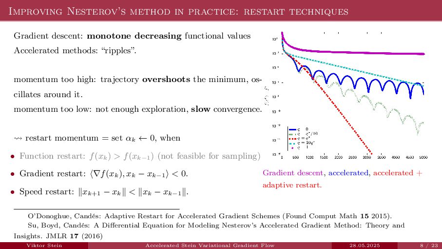[OC15] Brendan O’Donoghue and Emmanuel Candes, Adaptive restart for accelerated gradient schemes, Foundations of Computational Mathematics 15 (2015), 715–732. Viktor Stein Accelerated Stein Variational Gradient Flow 21.04.2025 1 / 3
23. References II [SBC16] Weijie Su, Stephen Boyd, and Emmanuel J Candes, A differential equation for modeling Nesterov’s accelerated gradient method: Theory and insights, Journal of Machine Learning Research 17 (2016), no. 153, 1–43. [WL22] Yifei Wang and Wuchen Li, Accelerated information gradient flow, Journal of Scientific Computing 90 (2022), 1–47. Viktor Stein Accelerated Stein Variational Gradient Flow 21.04.2025 2 / 3
24. Shameless plug: other works Interpolating between OT and KL regularized OT using Rényi Divergences Rényi divergence ̸∈ {f-div., Bregman div.}, α ∈ (0, 1) Rα (µ | ν) := 1 α − 1 ln X dµ dτ α dν dτ 1−α dτ , OTε,α (µ, ν) := min π∈Π(µ,ν) ⟨c, π⟩ + εRα (π | µ ⊗ ν) is a metric, where ε > 0, µ, ν ∈ P(X), X compact. OT(µ, ν) α↘0 ← − − − − or ε→0 OTε,α (µ, ν) α↗1 − − − → OTKL ε (µ, ν). In the works: debiased Rényi-Sinkhorn divergence OTε,α (µ, ν) − 1 2 OTε,α (µ, µ) − 1 2 OTε,α (ν, ν). W2 gradient flows of dK (·, ν)2 with K(x, y) := −|x − y| in 1D. Reformulation as maximal monotone inclu- sion Cauchy problem in L2 (0, 1) via quantile functions. Comprehensive description of solutions’ behav- ior, instantaneous measure-to-L∞ regular- ization, implicit Euler is simple. Viktor Stein Accelerated Stein Variational Gradient Flow 21.04.2025 3 / 3 −1 −0.5 0.5 1 1.5 2 1 2 3 µ0 8 6 4 2 0 2 4 6 8 0.00 0.05 0.10 0.15 0.20 0.25 0.30 0.35 0.40 Iteration 0 initial target explicit implicit