Some comments on probability theory

Transcript

1. SOME COMMENTS ON PROBABILITY THEORY Bagus Tris Atmaja 114-D9818
2. Outline 2.1.Noise and Random Variables 2.2.Correlated Data 2.3.Function of Random Variables 2.4.Gaussian Distribution 2.5. Testing the Assumption of Gaussian Statistics 2.6.Confidence Interval
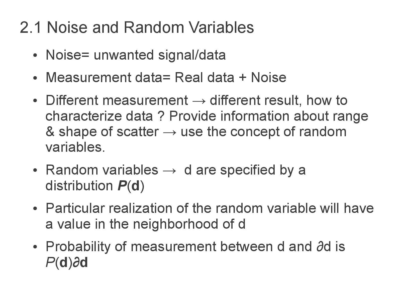
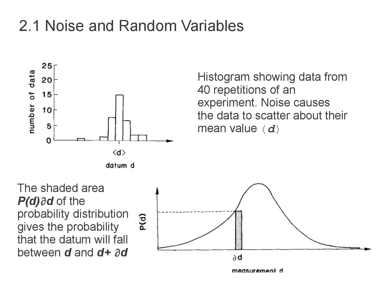
3. • Noise= unwanted signal/data • Measurement data= Real data + Noise • Different measurement → different result, how to characterize data ? Provide information about range & shape of scatter → use the concept of random variables. • Random variables → d are specified by a distribution P(d) • Particular realization of the random variable will have a value in the neighborhood of d • Probability of measurement between d and ∂d is P(d)∂d 2.1 Noise and Random Variables
4. 2.1 Noise and Random Variables The shaded area P(d)d of the probability distribution gives the probability that the datum will fall between d and d+ d Histogram showing data from 40 repetitions of an experiment. Noise causes the data to scatter about their mean value 〈d〉
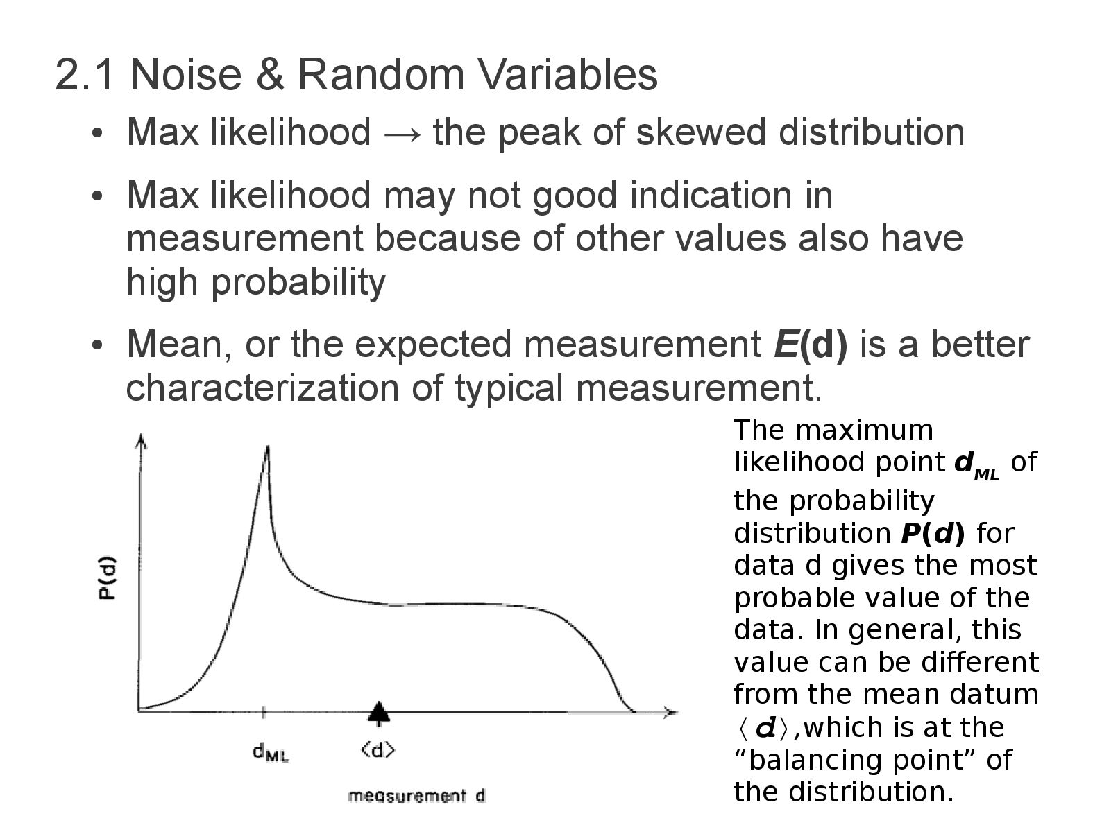
5. 2.1 Noise & Random Variables • Max likelihood → the peak of skewed distribution • Max likelihood may not good indication in measurement because of other values also have high probability • Mean, or the expected measurement E(d) is a better characterization of typical measurement. The maximum likelihood point d ML of the probability distribution P(d) for data d gives the most probable value of the data. In general, this value can be different from the mean datum 〈d〉,which is at the “balancing point” of the distribution.
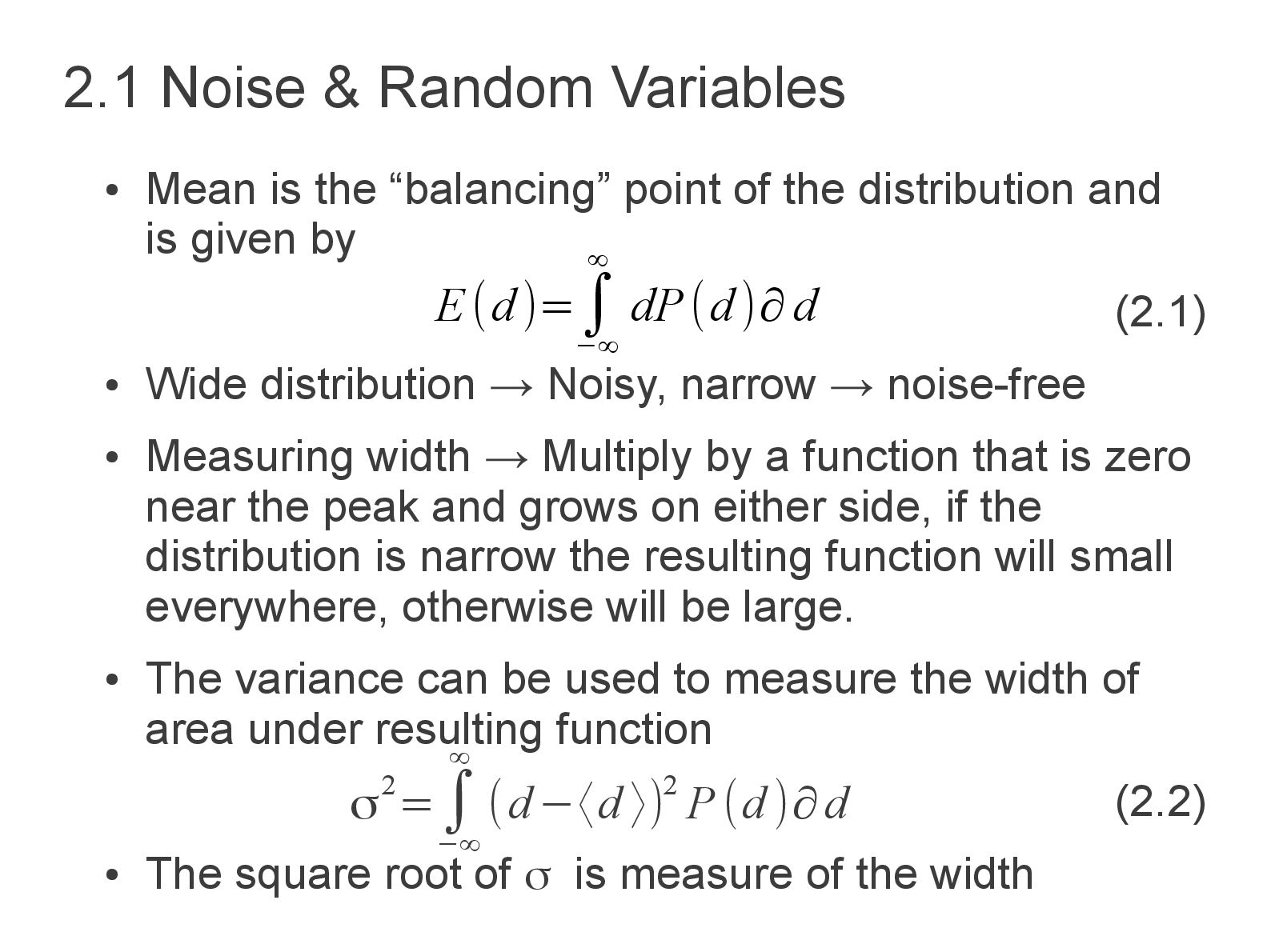
6. 2.1 Noise & Random Variables • Mean is the “balancing” point of the distribution and is given by (2.1) • Wide distribution → Noisy, narrow → noise-free • Measuring width → Multiply by a function that is zero near the peak and grows on either side, if the distribution is narrow the resulting function will small everywhere, otherwise will be large. • The variance can be used to measure the width of area under resulting function (2.2) • The square root of σ is measure of the width E(d)=∫ −∞ ∞ dP(d)∂ d σ2=∫ −∞ ∞ (d−〈d 〉)2 P(d )∂d
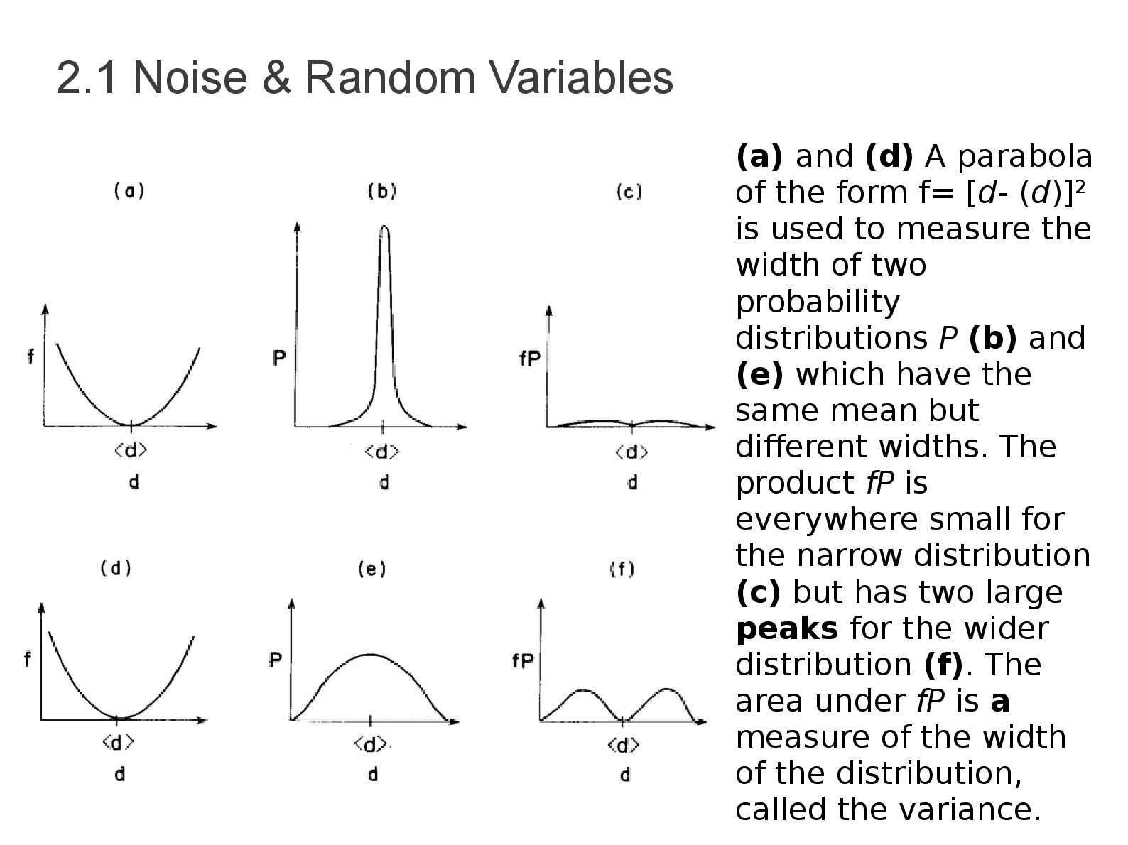
7. 2.1 Noise & Random Variables (a) and (d) A parabola of the form f= [d- (d)]2 is used to measure the width of two probability distributions P (b) and (e) which have the same mean but different widths. The product fP is everywhere small for the narrow distribution (c) but has two large peaks for the wider distribution (f). The area under fP is a measure of the width of the distribution, called the variance.
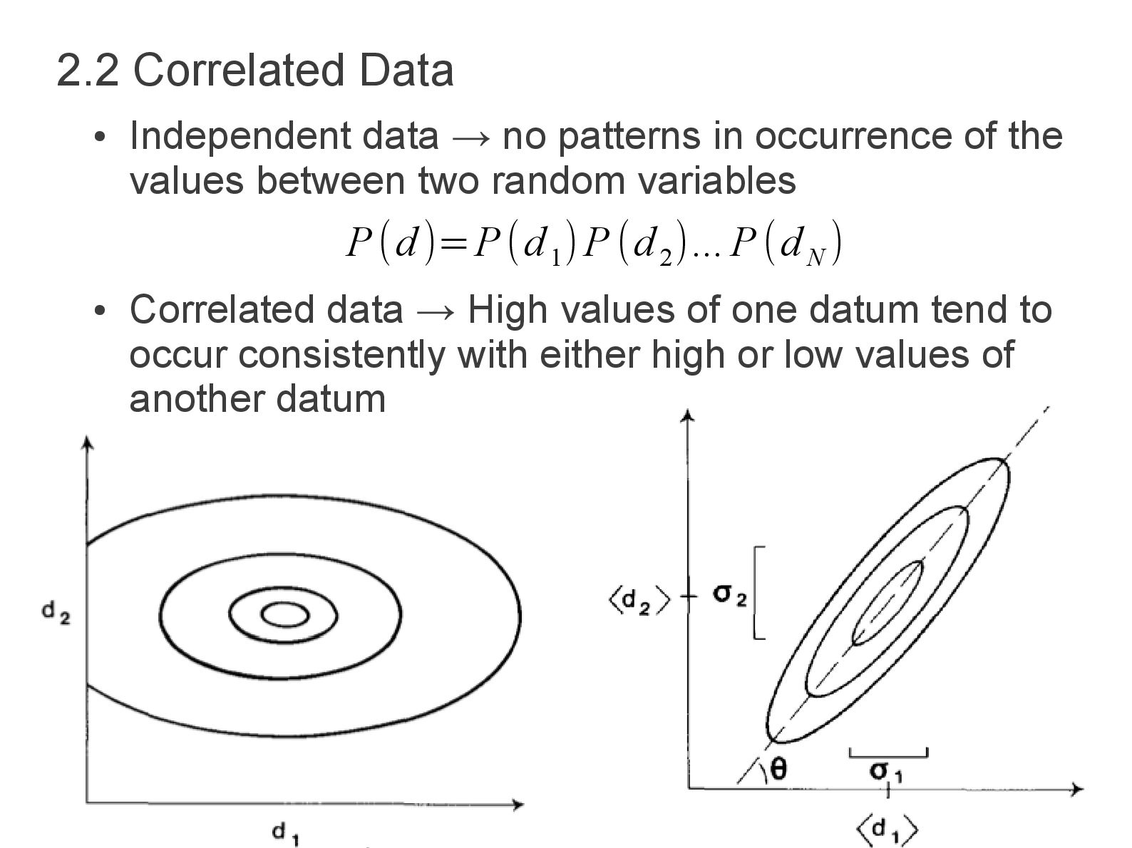
8. 2.2 Correlated Data • Independent data → no patterns in occurrence of the values between two random variables • Correlated data → High values of one datum tend to occur consistently with either high or low values of another datum P(d)=P(d 1 )P(d 2 )... P(d N )
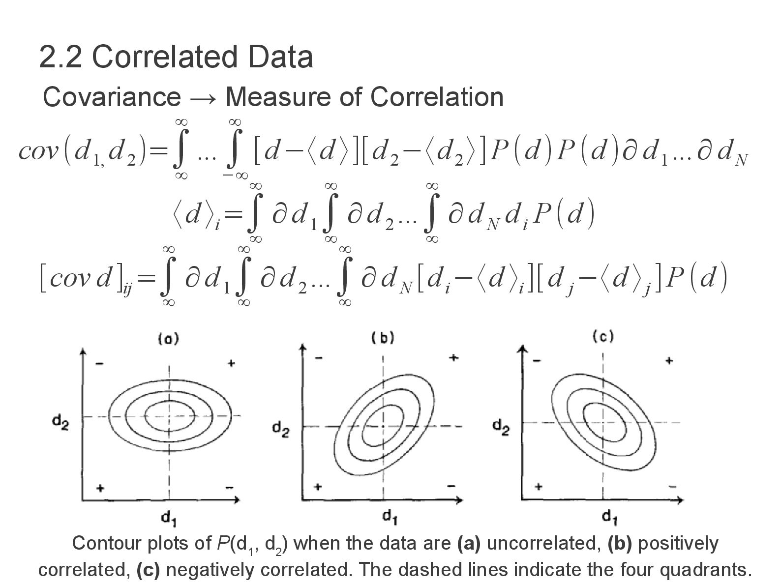
9. cov(d 1, d 2 )=∫ ∞ ∞ ...∫ −∞ ∞ [d−〈d 〉][d 2 −〈d 2 〉]P(d)P(d )∂ d 1 ...∂ d N 〈d 〉 i =∫ ∞ ∞ ∂d 1 ∫ ∞ ∞ ∂d 2 ...∫ ∞ ∞ ∂d N d i P(d) [cov d ]ij =∫ ∞ ∞ ∂d 1 ∫ ∞ ∞ ∂d 2 ...∫ ∞ ∞ ∂d N [d i −〈d 〉i ][d j −〈d 〉j ]P(d) 2.2 Correlated Data Covariance → Measure of Correlation Contour plots of P(d 1 , d 2 ) when the data are (a) uncorrelated, (b) positively correlated, (c) negatively correlated. The dashed lines indicate the four quadrants.
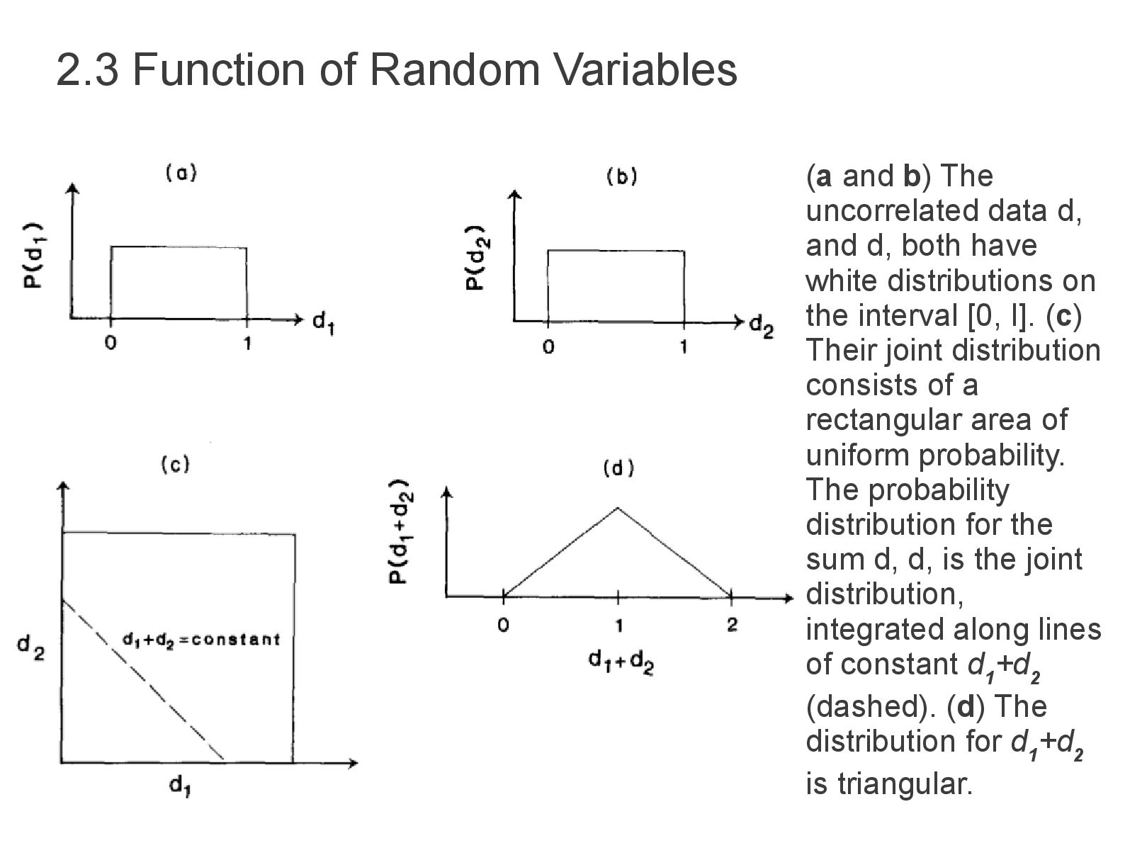
10. • Basic premise = data and model parameters are related • Estimation of model parameters are random variable described by distribution P (mest) • Whether or not true model parameters are random variables depend on the problem. • If the distribution of data is known then the distribution for any function of data including model parameters can be found. • The joint distribution of two uncorrelated data is triangular as will be explained on the next slide. 2.2 Function of Random Variables
11. 2.3 Function of Random Variables (a and b) The uncorrelated data d, and d, both have white distributions on the interval [0, I]. (c) Their joint distribution consists of a rectangular area of uniform probability. The probability distribution for the sum d, d, is the joint distribution, integrated along lines of constant d 1 +d 2 (dashed). (d) The distribution for d 1 +d 2 is triangular.
12. • Performing the line integral on triangular in case of linear function m=Md+v (M:matrix and V: vector) can be simplified by stating mean and covariance, • Consider model parameter m 1 which is mean of data, • That is, M = [ 1, 1, 1, . . . , 1]/N and v = 0. Suppose that the data are uncorrelated and all have the same mean (d) and variance σ d 2.. • Hence model parameter m 1 has distribution P (m 1 ) denan mean m 1 =d dan variance σ d 2=σ d 2 /N. So, m 1 close to the true mean is proportional to N-1/2 2.3 Function of Random Variables 〈d 〉=M 〈d 〉+v [cov m]=M [cov d ] MT 〈m 1 〉=M 〈d 〉 (m 1 )=M [cov d ] MT =σ d 2 /N m 1 =1/N ∑ i N d i =(1/N )[1,1,1,...,1]d
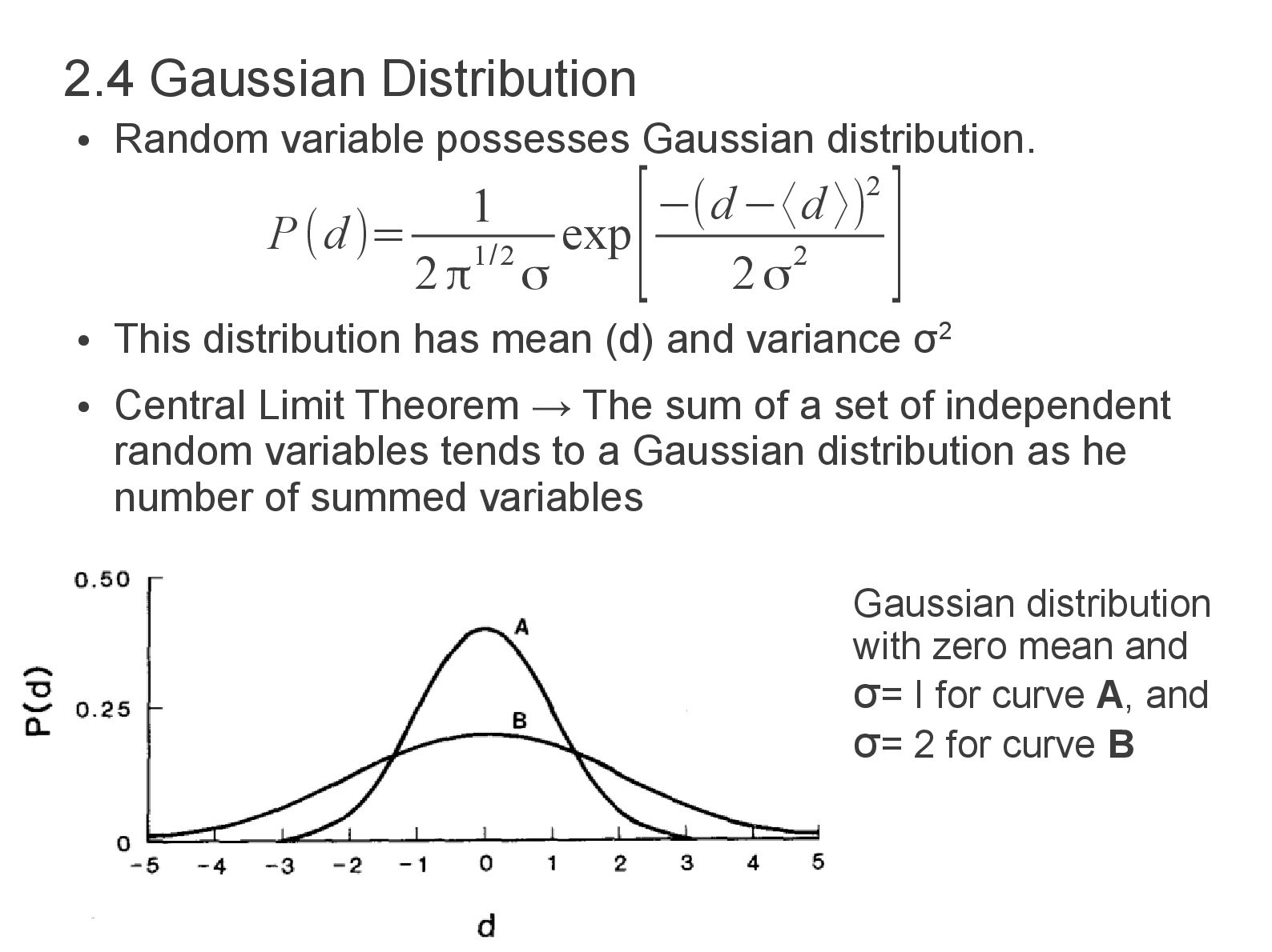
13. • Random variable possesses Gaussian distribution. • This distribution has mean (d) and variance σ2 • Central Limit Theorem → The sum of a set of independent random variables tends to a Gaussian distribution as he number of summed variables 2.4 Gaussian Distribution P(d)= 1 2π1/2 σ exp [−(d−〈d 〉)2 2σ2 ] Gaussian distribution with zero mean and σ= I for curve A, and σ= 2 for curve B
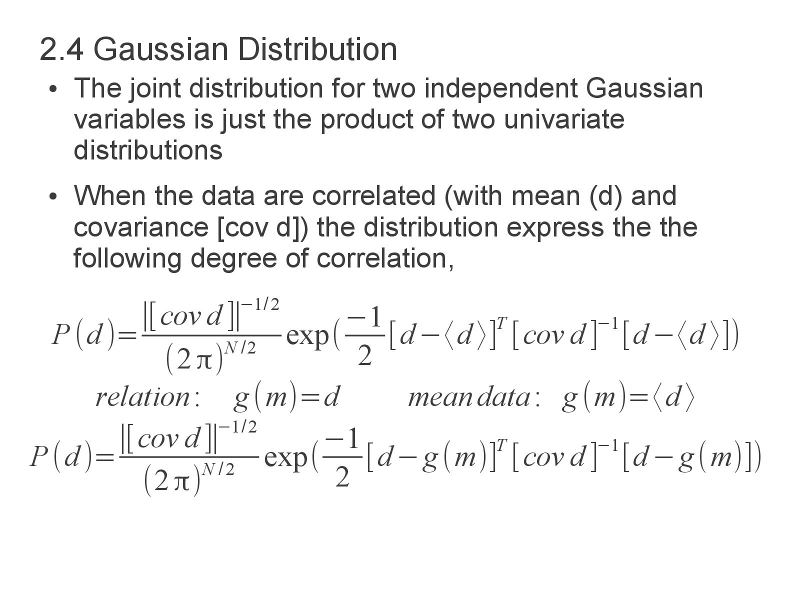
14. • The joint distribution for two independent Gaussian variables is just the product of two univariate distributions • When the data are correlated (with mean (d) and covariance [cov d]) the distribution express the the following degree of correlation, 2.4 Gaussian Distribution P(d)= ∣[cov d ]∣−1/2 (2π)N /2 exp( −1 2 [d−〈d〉]T [cov d]−1[d−〈d 〉]) relation: g(m)=d meandata: g(m)=〈d〉 P(d)= ∣[cov d]∣−1/2 (2π)N /2 exp( −1 2 [d−g(m)]T [cov d]−1[d−g(m)])
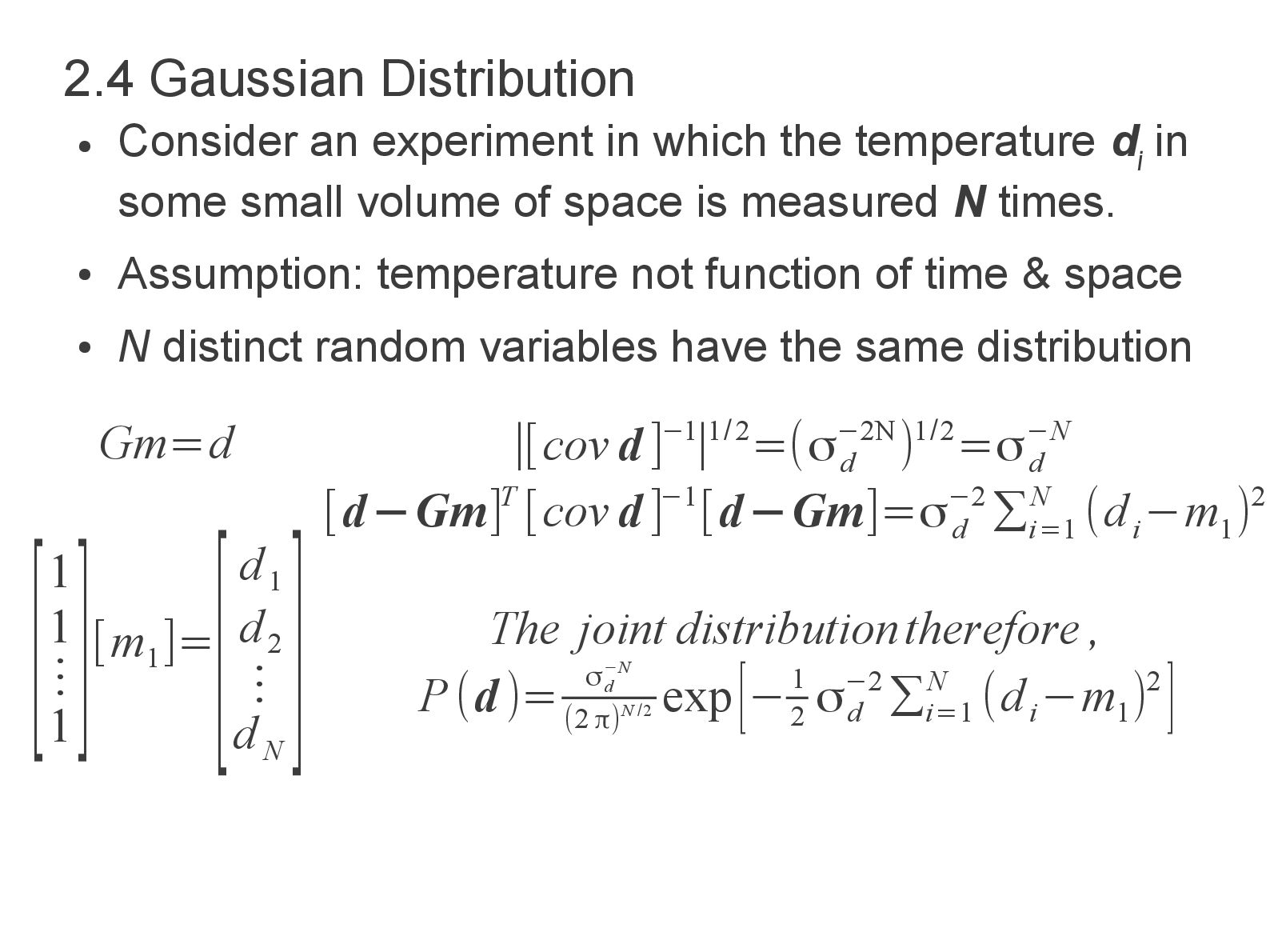
15. • Consider an experiment in which the temperature d i in some small volume of space is measured N times. • Assumption: temperature not function of time & space • N distinct random variables have the same distribution 2.4 Gaussian Distribution Gm=d [1 1 ⋮ 1 ][m 1 ]= [d 1 d 2 ⋮ d N ] ∣[cov d ]−1∣1/2=(σ d −2N)1/2=σ d −N [d−Gm]T [cov d ]−1[d−Gm]=σ d −2 ∑ i=1 N (d i −m 1 )2 The joint distributiontherefore , P(d )= σ d −N (2 π)N /2 exp[−1 2 σd −2 ∑i=1 N (d i −m 1 )2 ]
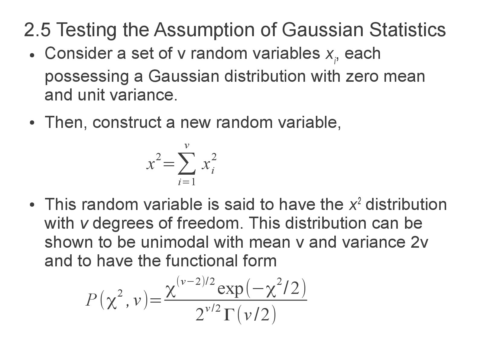
16. • Consider a set of v random variables x i , each possessing a Gaussian distribution with zero mean and unit variance. • Then, construct a new random variable, • This random variable is said to have the x2 distribution with v degrees of freedom. This distribution can be shown to be unimodal with mean v and variance 2v and to have the functional form 2.5 Testing the Assumption of Gaussian Statistics x2=∑ i=1 v x i 2 P(χ2 ,v)= χ(v−2)/2 exp(−χ2/2) 2v/2 Γ(v/2)
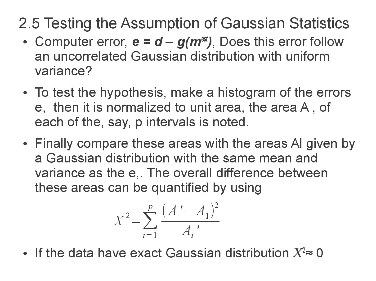
17. 2.5 Testing the Assumption of Gaussian Statistics X 2=∑ i=1 p (A'−A 1 )2 A i ' • Computer error, e = d – g(mest), Does this error follow an uncorrelated Gaussian distribution with uniform variance? • To test the hypothesis, make a histogram of the errors e, then it is normalized to unit area, the area A , of each of the, say, p intervals is noted. • Finally compare these areas with the areas Al given by a Gaussian distribution with the same mean and variance as the e,. The overall difference between these areas can be quantified by using • If the data have exact Gaussian distribution X2≈ 0
18. • X2 will not be zero since there are always random fluctuations • Need to inquire whether the X2 measured for any particular data set is sufficiently far from zero that it is improbable that the data follow the Gaussian distribution. • Compute the theoretical distribution of X2 and seeing whether X obs 2 is probable. • Data not follow the distribution → values greater than or equal to X obs 2 occur less than 5% of the time. • χ2 test → test whether the data follow any given distribution or not 2.5 Testing the Assumption of Gaussian Statistics
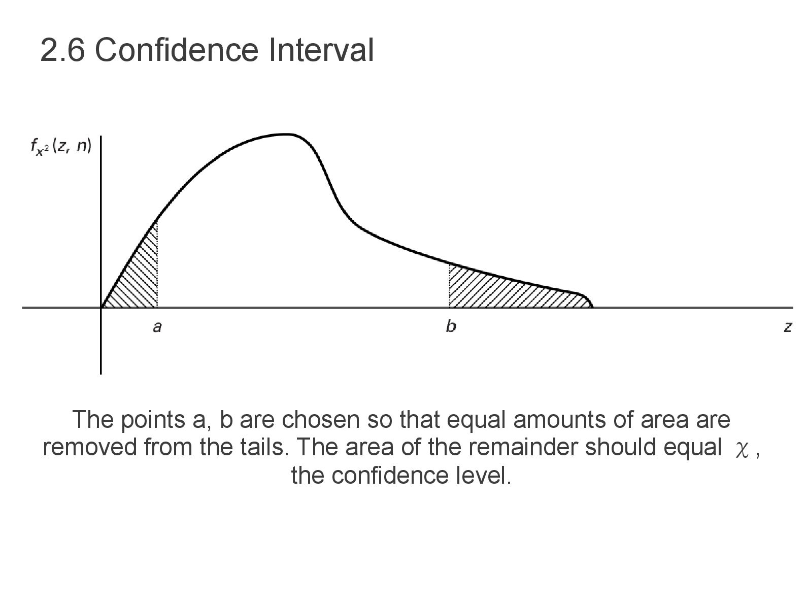
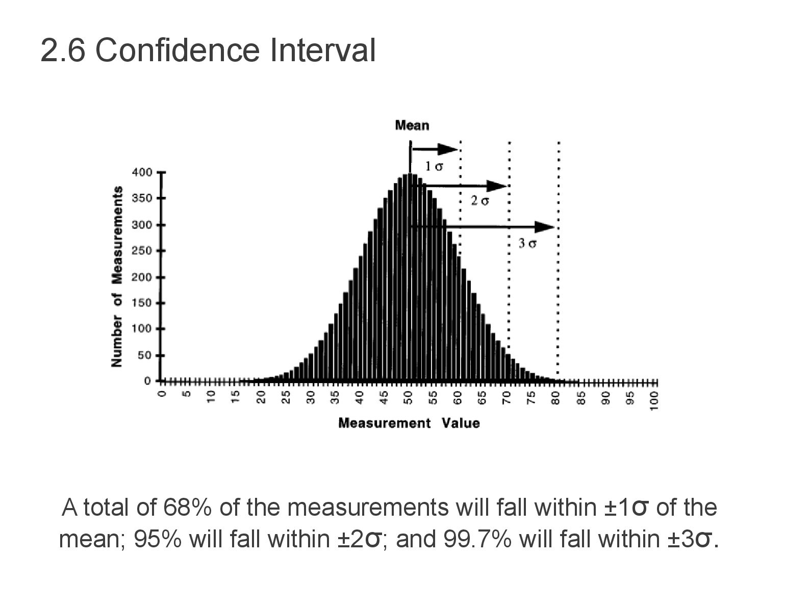
19. • The confidence of a particular observation is the probability that one realization of the random variable falls within a specified distance of the true mean. Therefore it is related to distribution in area P(d). • Distributions with large variances will also tend to have large confidence intervals (related but not direct). • For 95% confidence interval, 5% area under pdf is omitted or ( 2.5% each tail, lower a & upper b bound). • For random variable with σ= 1, then if a realization of that variable has the value 50, a 95% mean the random variable lies between 48 and 52 (a to b or (d)=50±2). • The more complicated the distribution, the more difficult to chose an appropriate shape and calculate the probability within it. 2.6 Confidence Interval
20. 2.6 Confidence Interval The points a, b are chosen so that equal amounts of area are removed from the tails. The area of the remainder should equal χ, the confidence level.
21. 2.6 Confidence Interval A total of 68% of the measurements will fall within ±1σ of the mean; 95% will fall within ±2σ; and 99.7% will fall within ±3σ.