Count-Min Sketch, Bloom Filter, TopK: Efficient probabilistic data structures

A Count-Min Sketch, a Bloom Filter, and a TopK might sound fancy, but they’re just smart ways to work with huge amounts of data using very little memory.

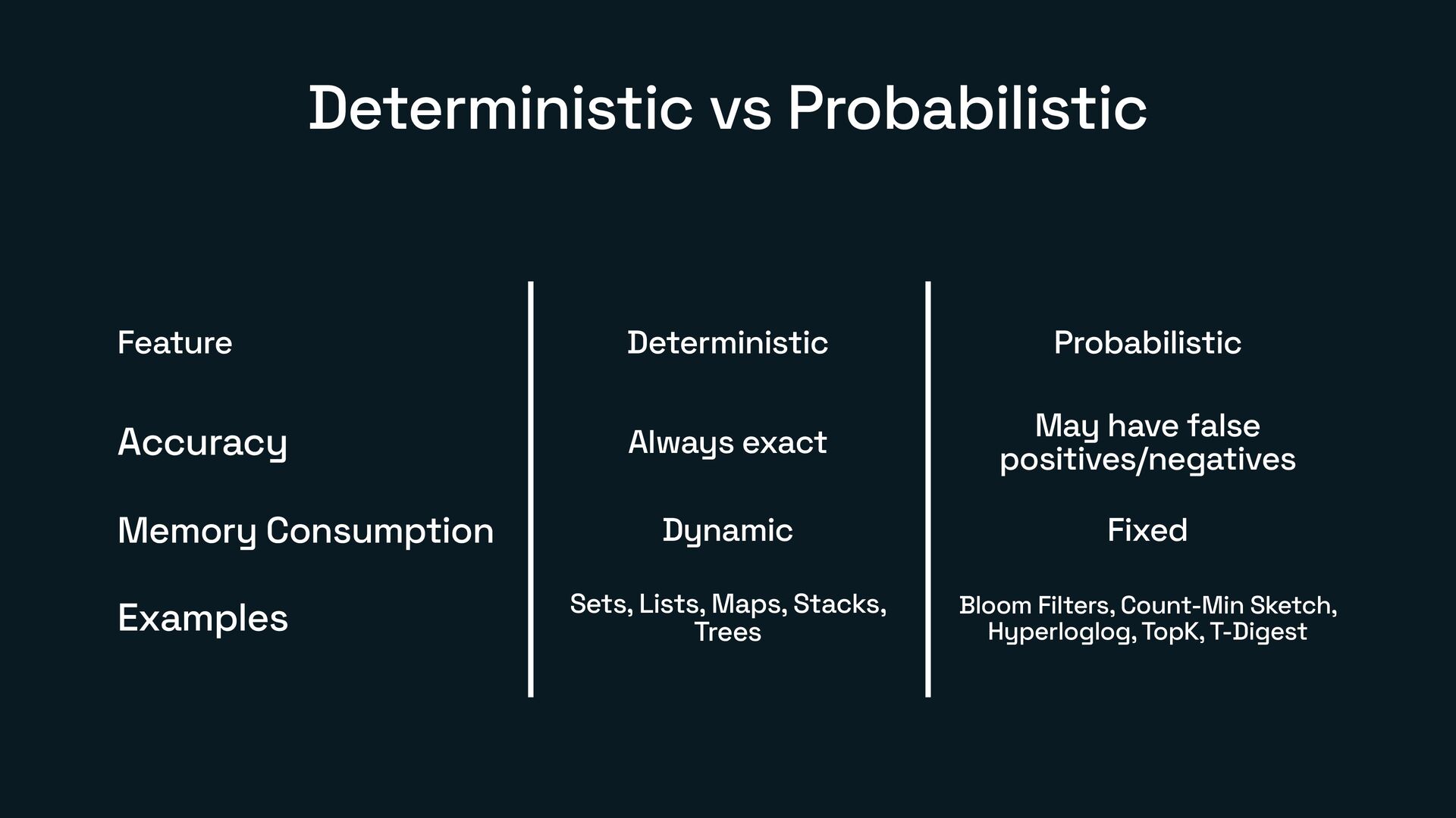
In this talk, we’ll explore three powerful probabilistic data structures that trade a bit of accuracy for a lot of speed and scalability. You’ll learn:

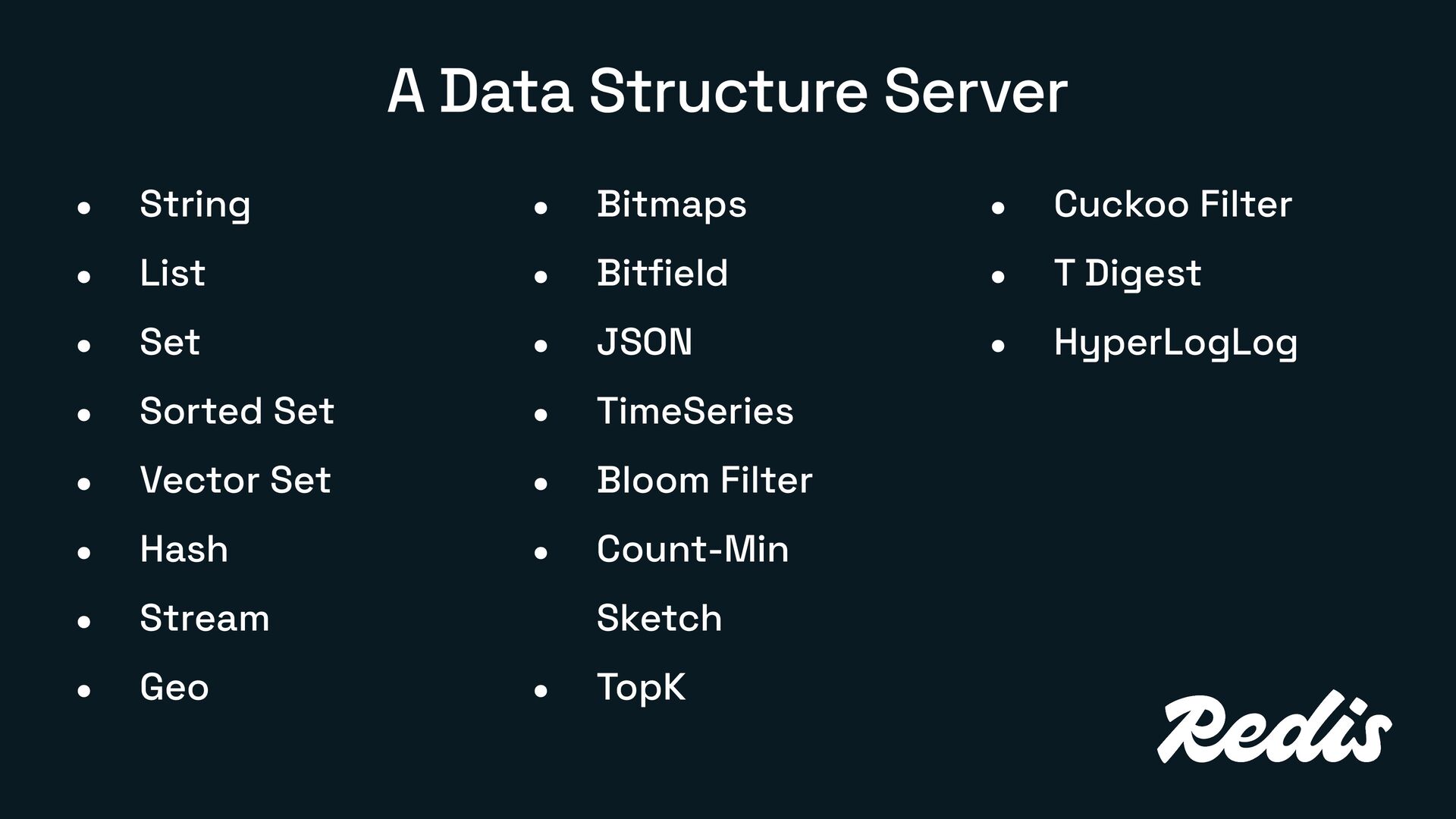
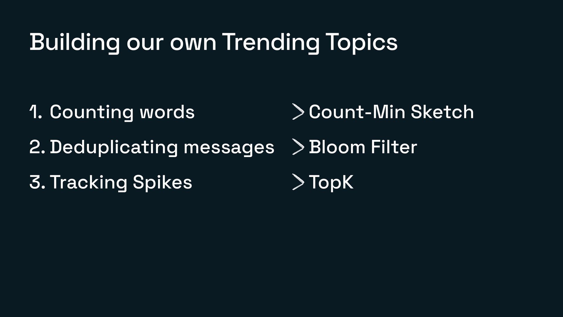
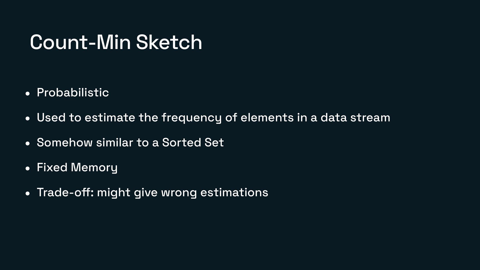
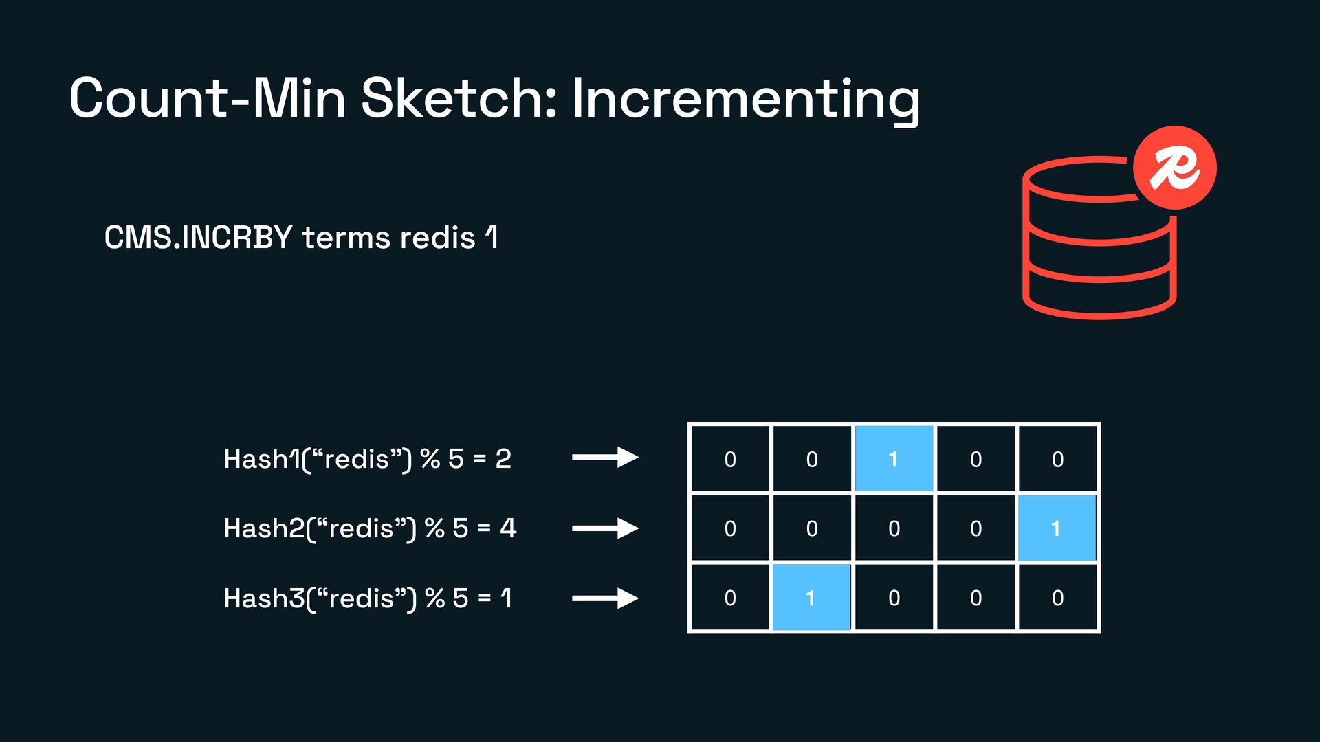
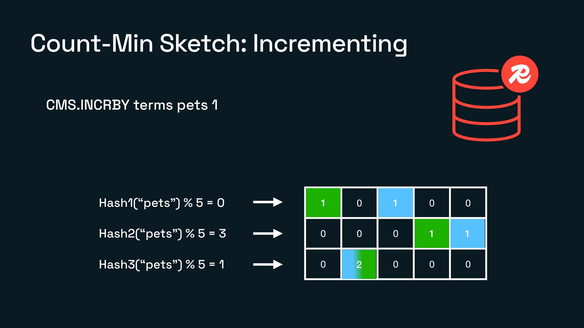
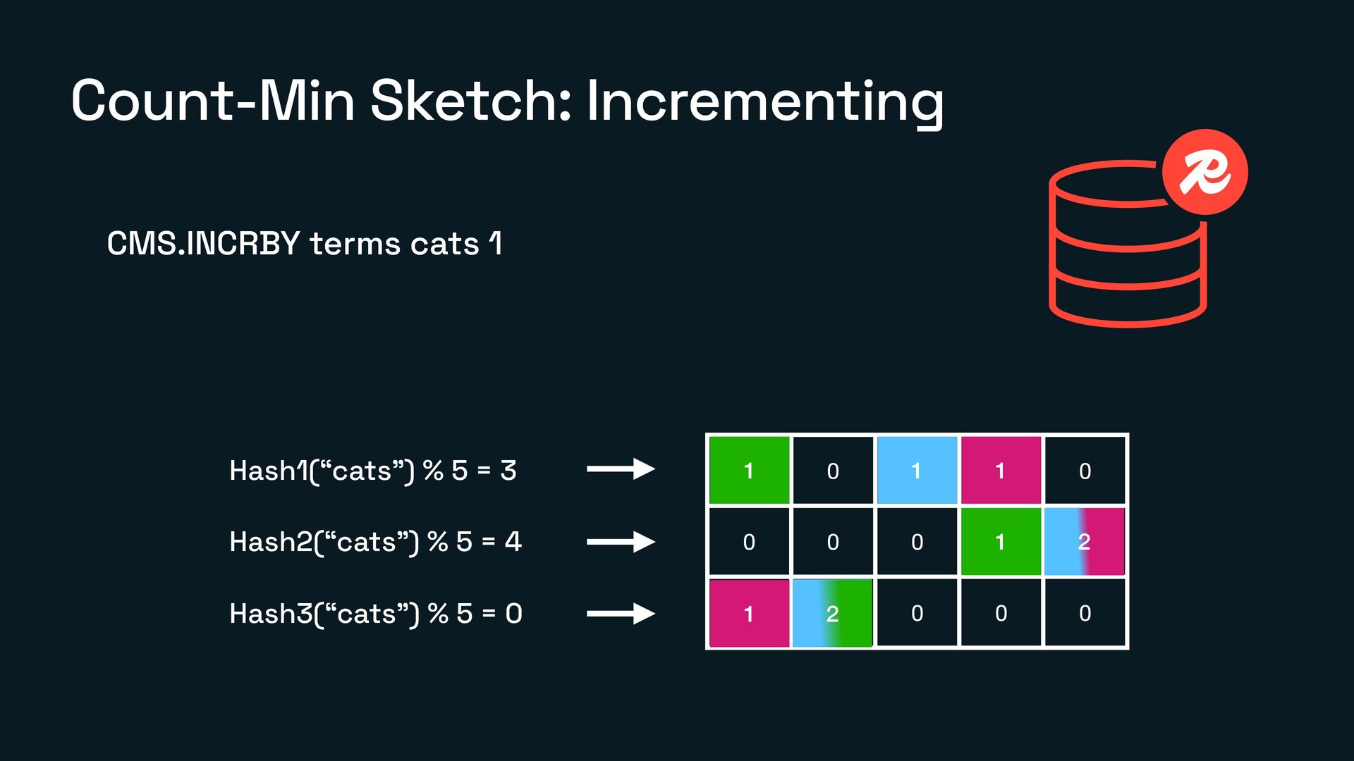
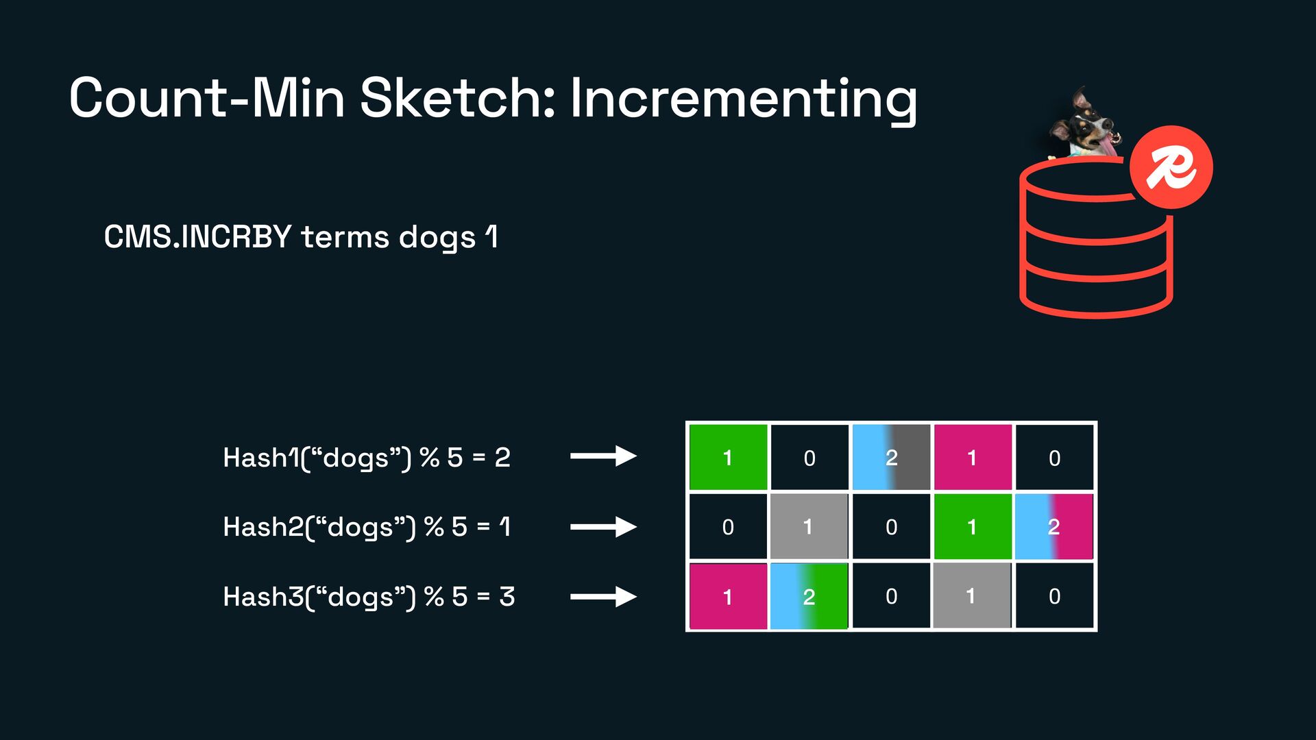
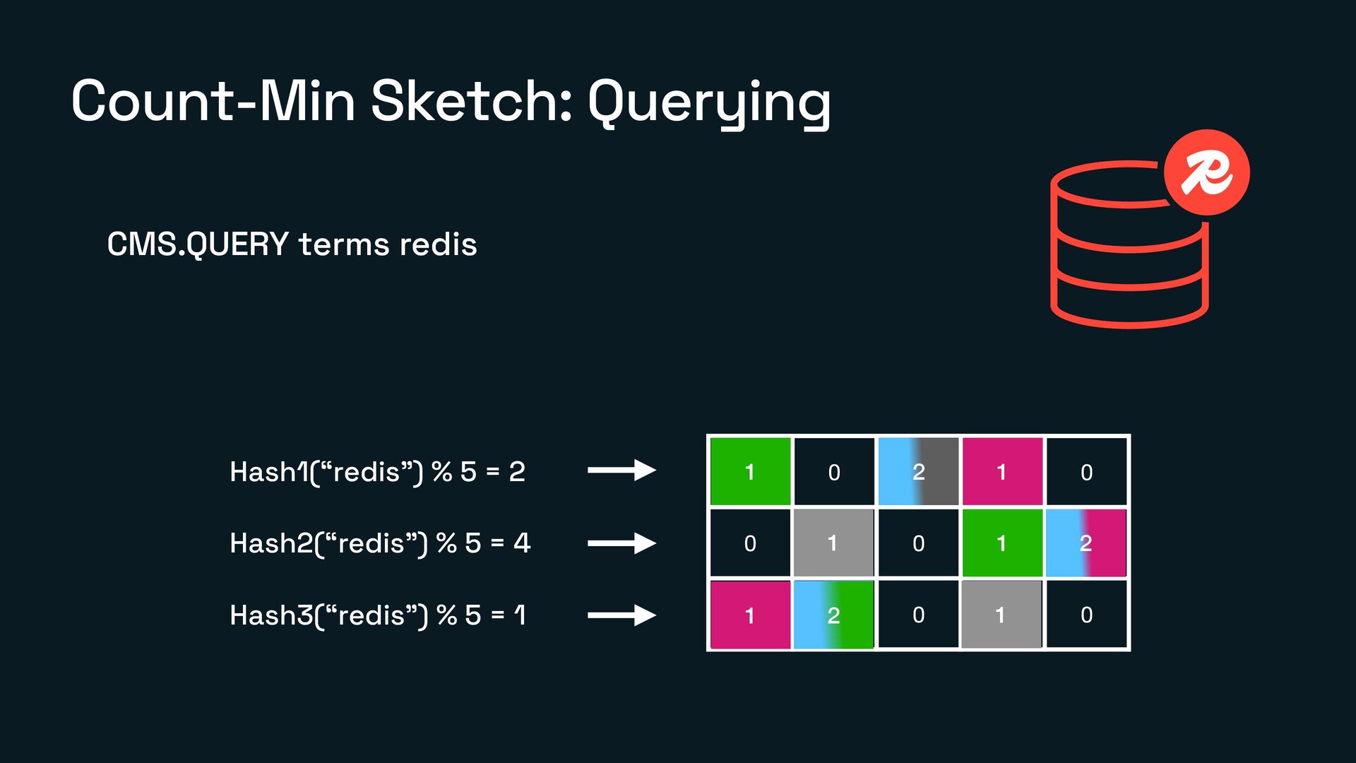
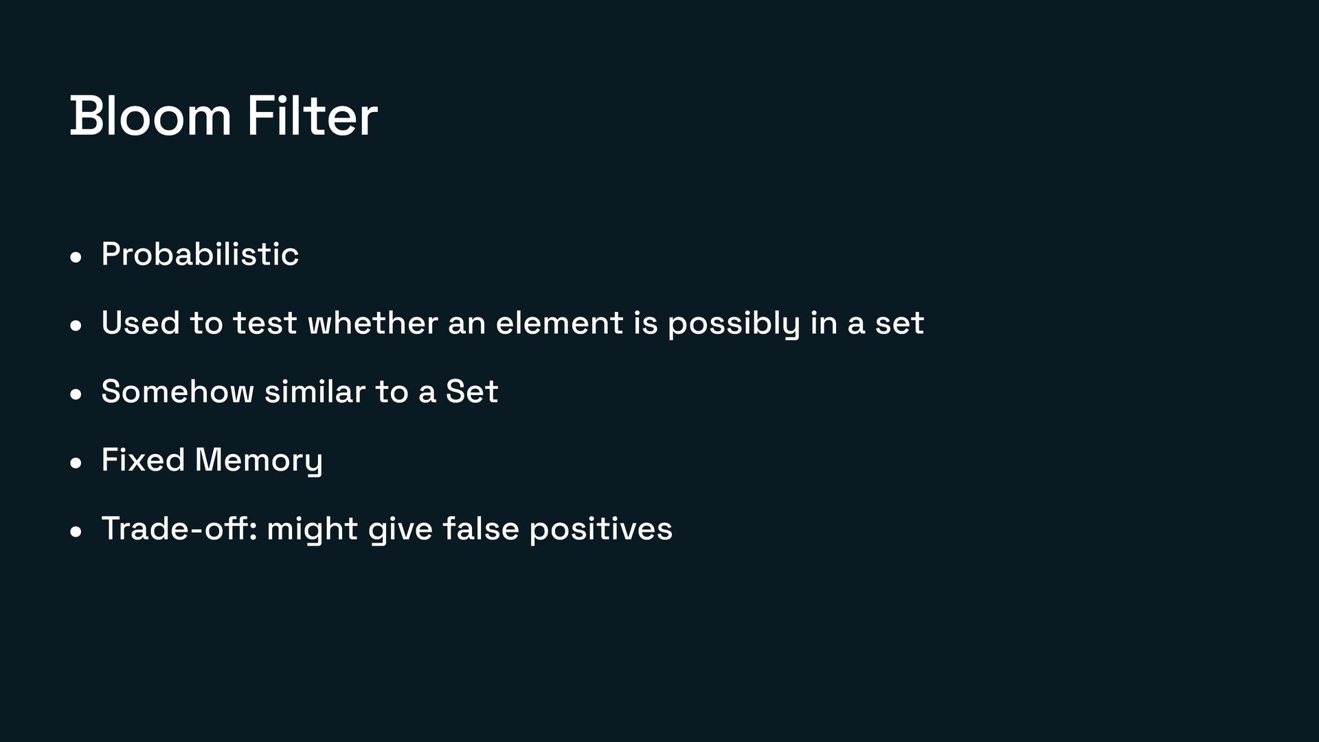
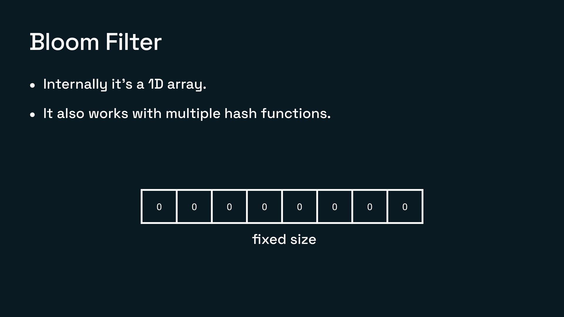
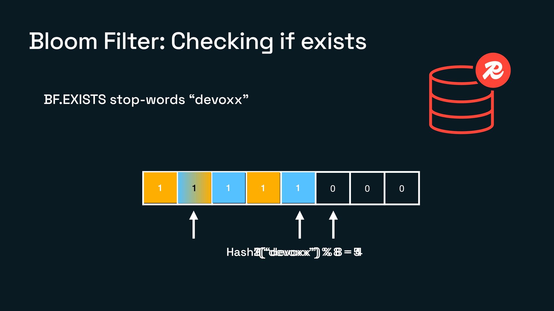
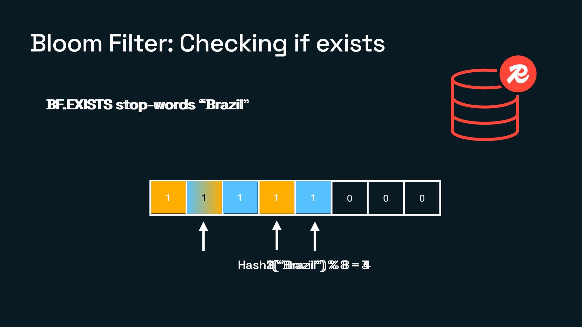
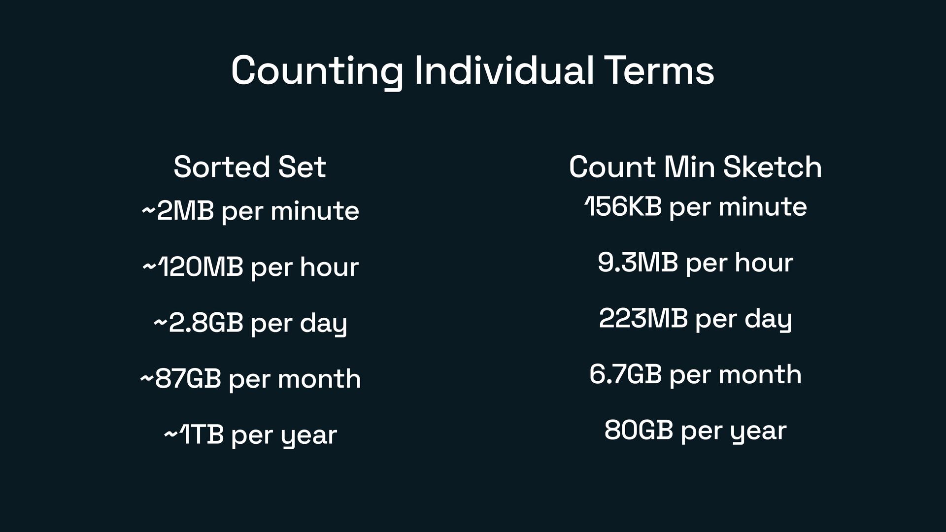
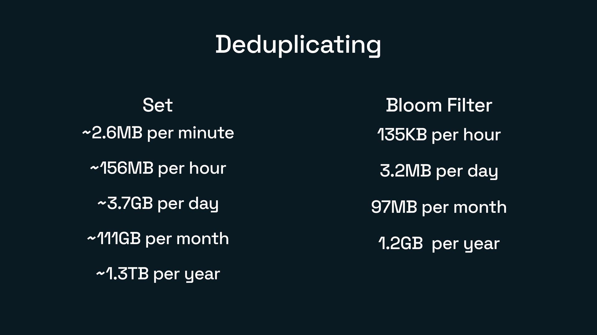
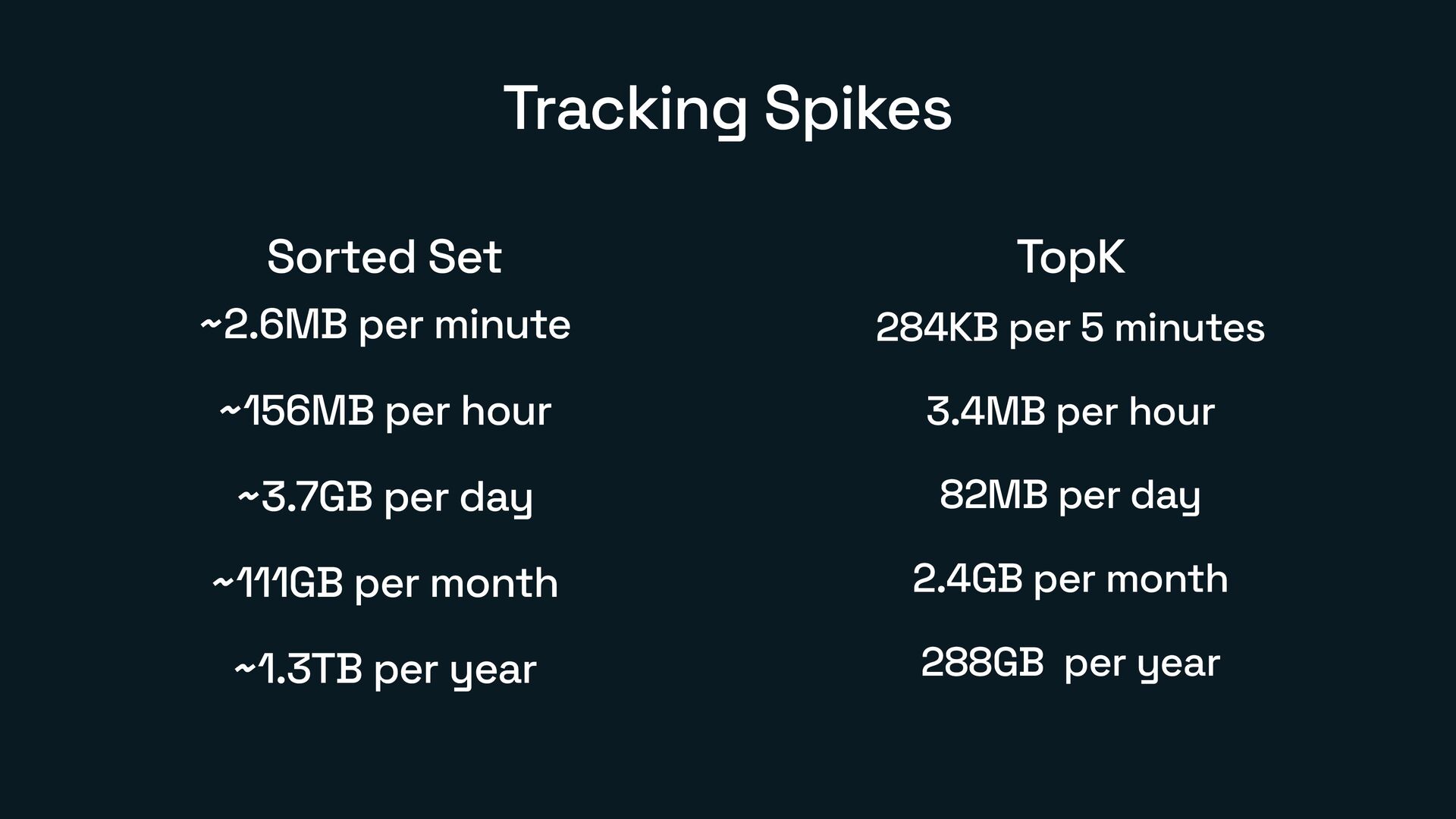
What Count-Min Sketch, Bloom Filter, and TopK actually are
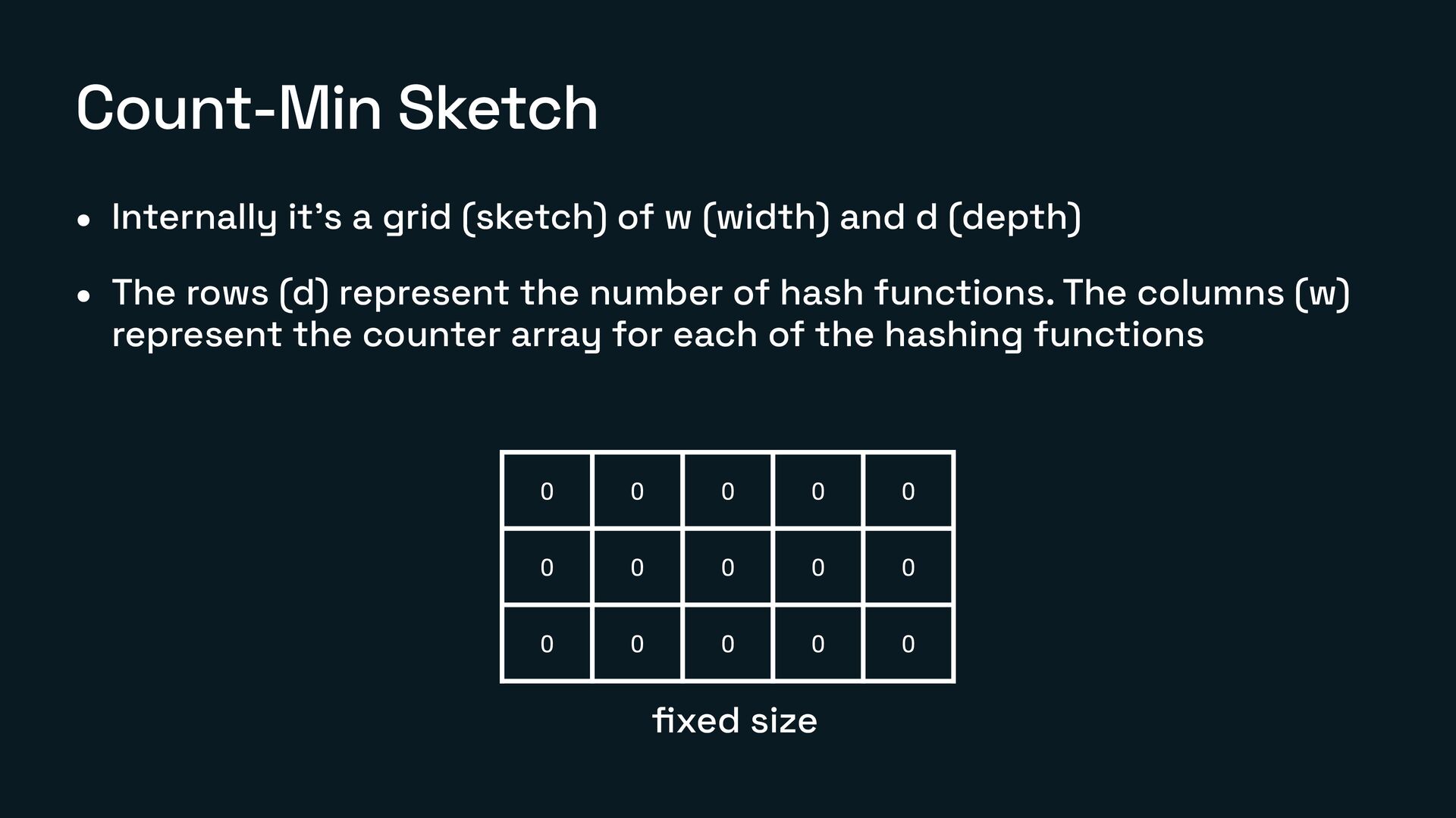
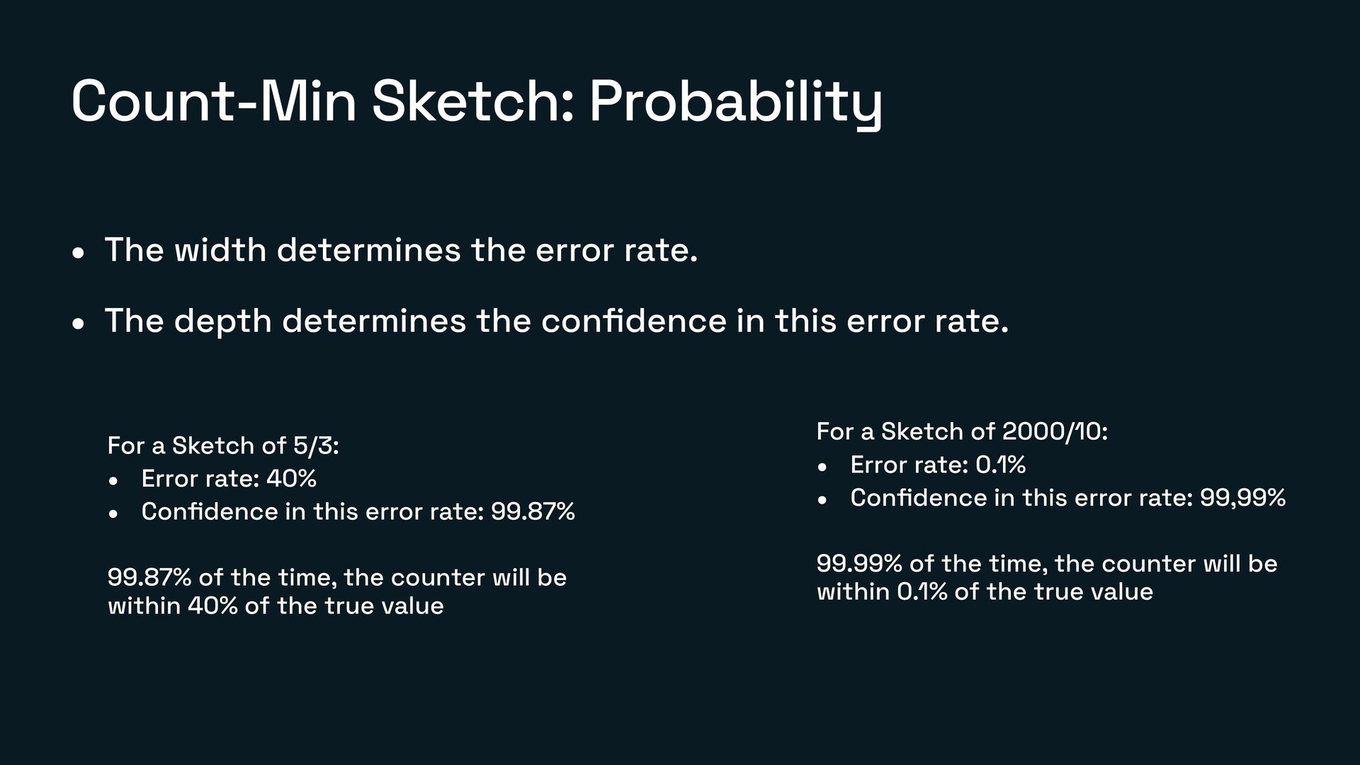
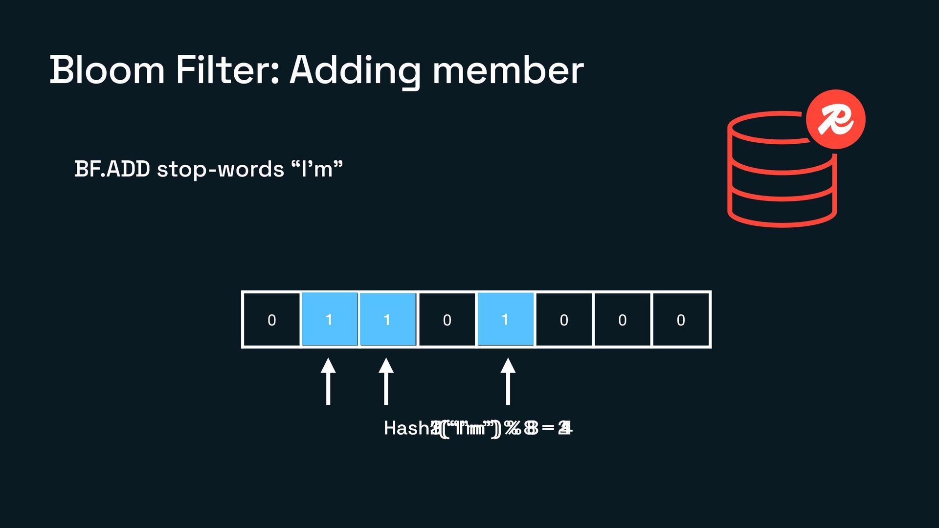
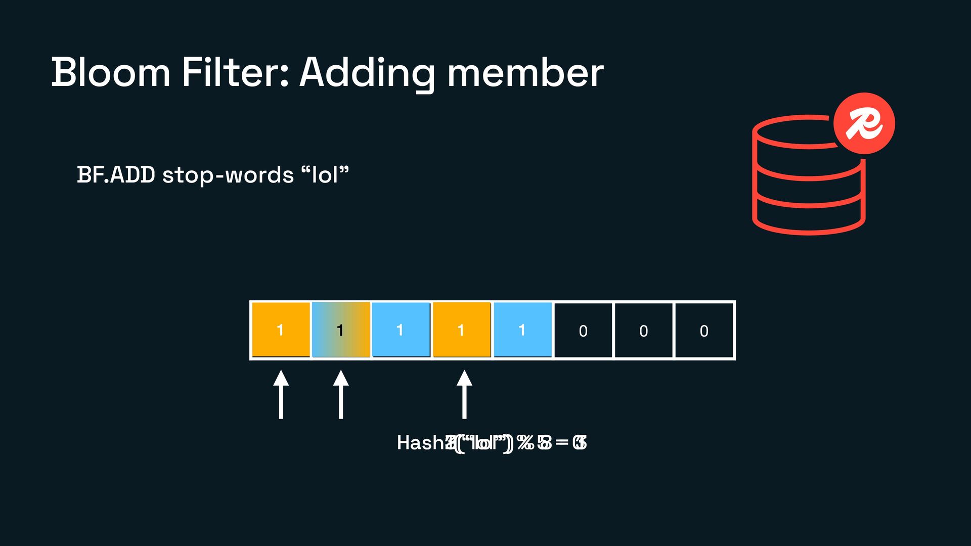
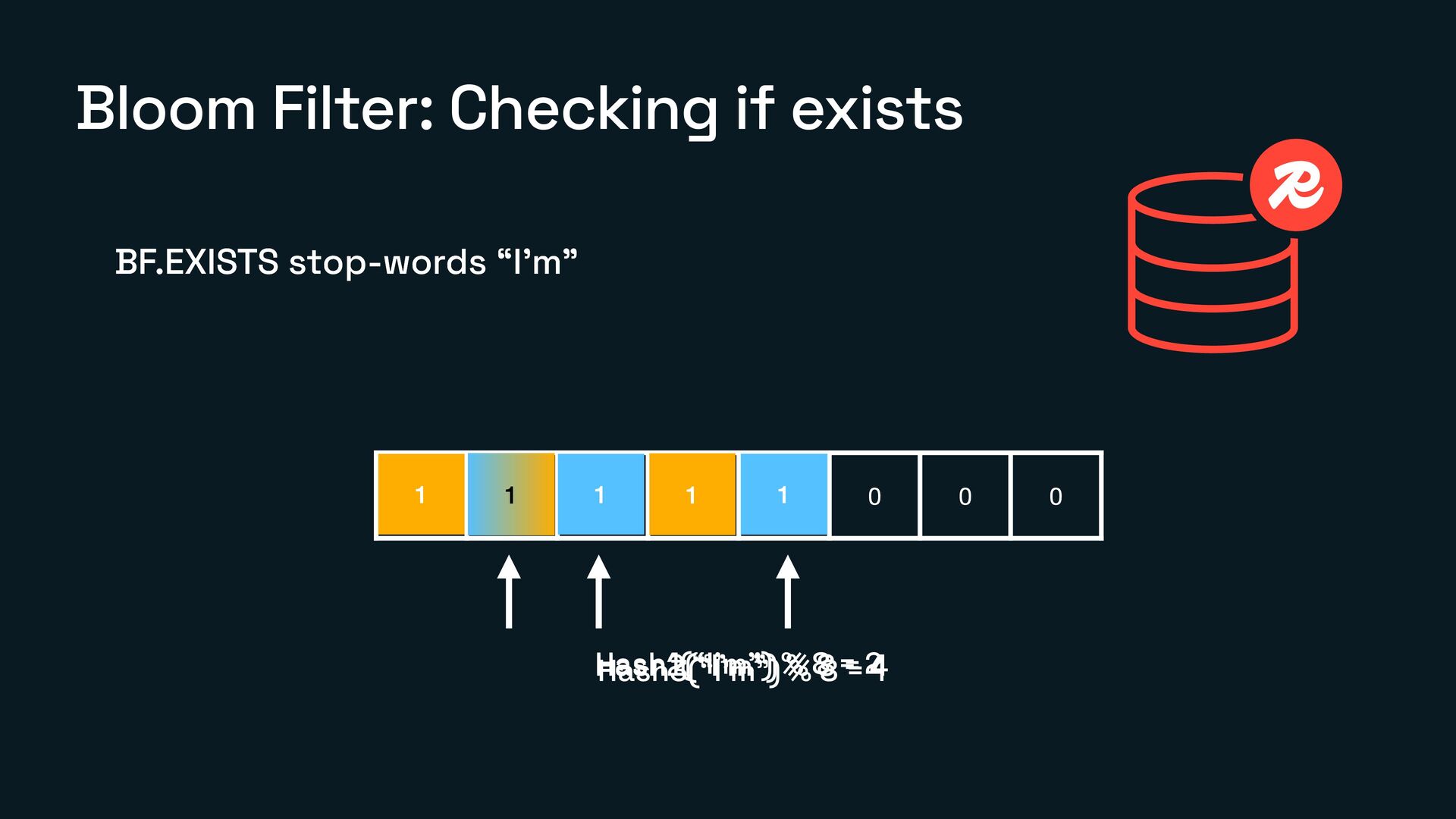
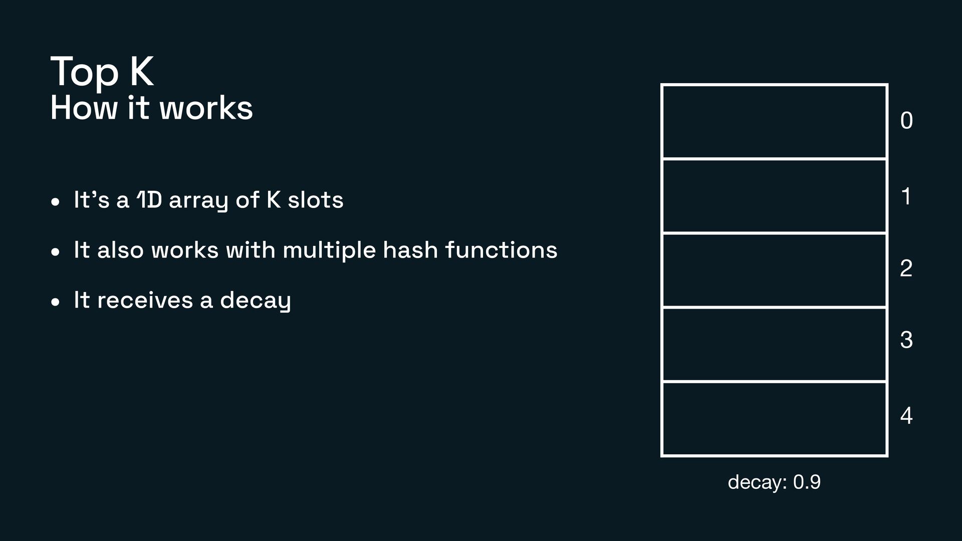
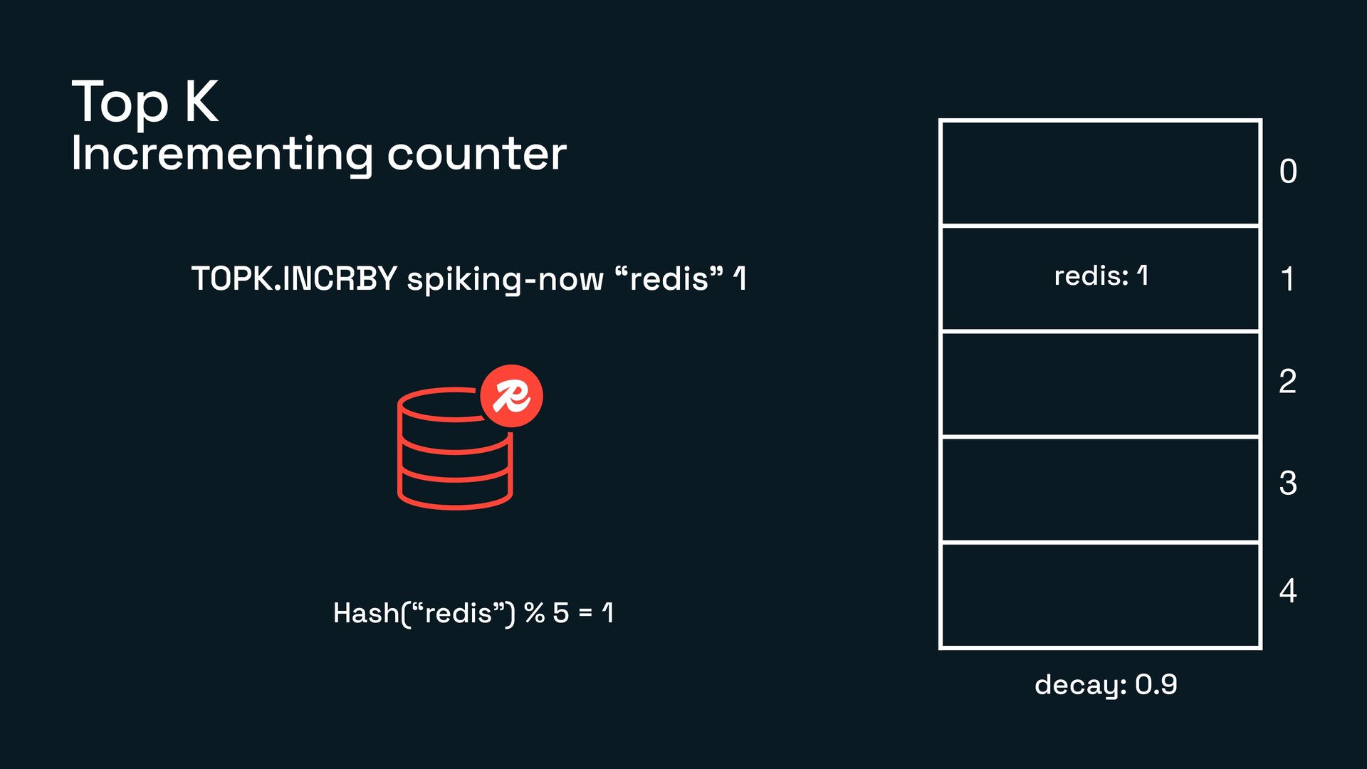
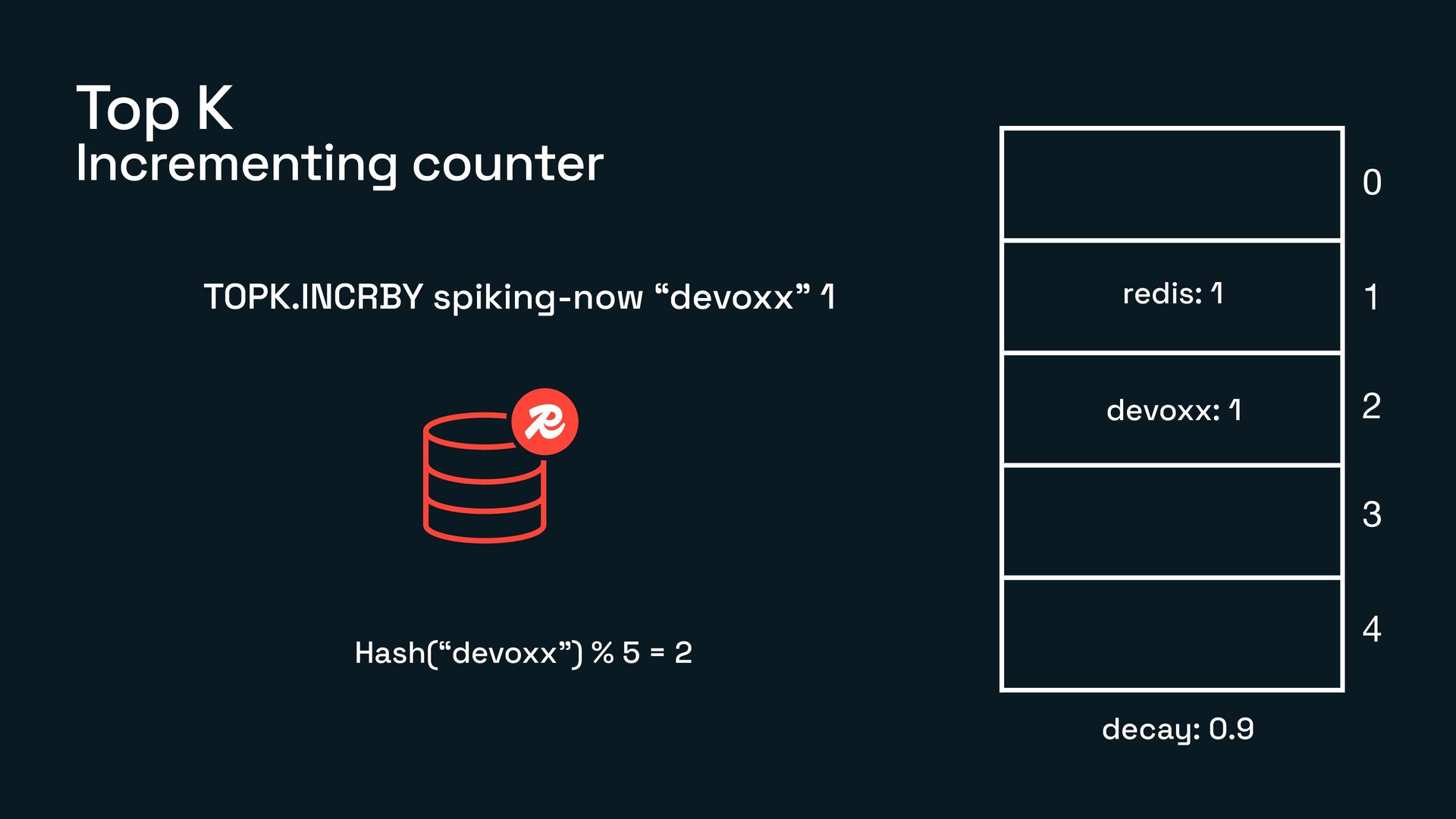
How each of them works under the hood
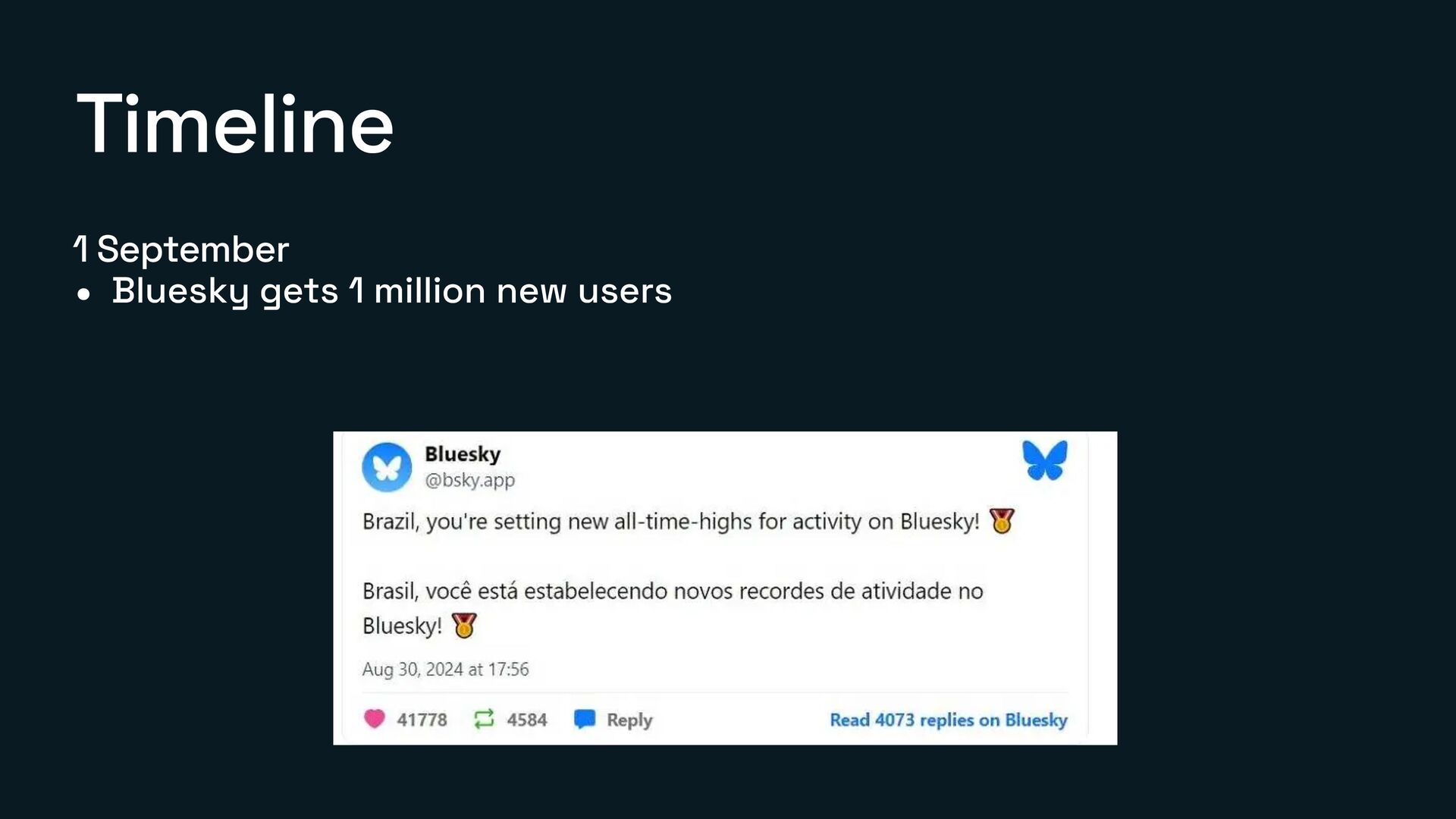
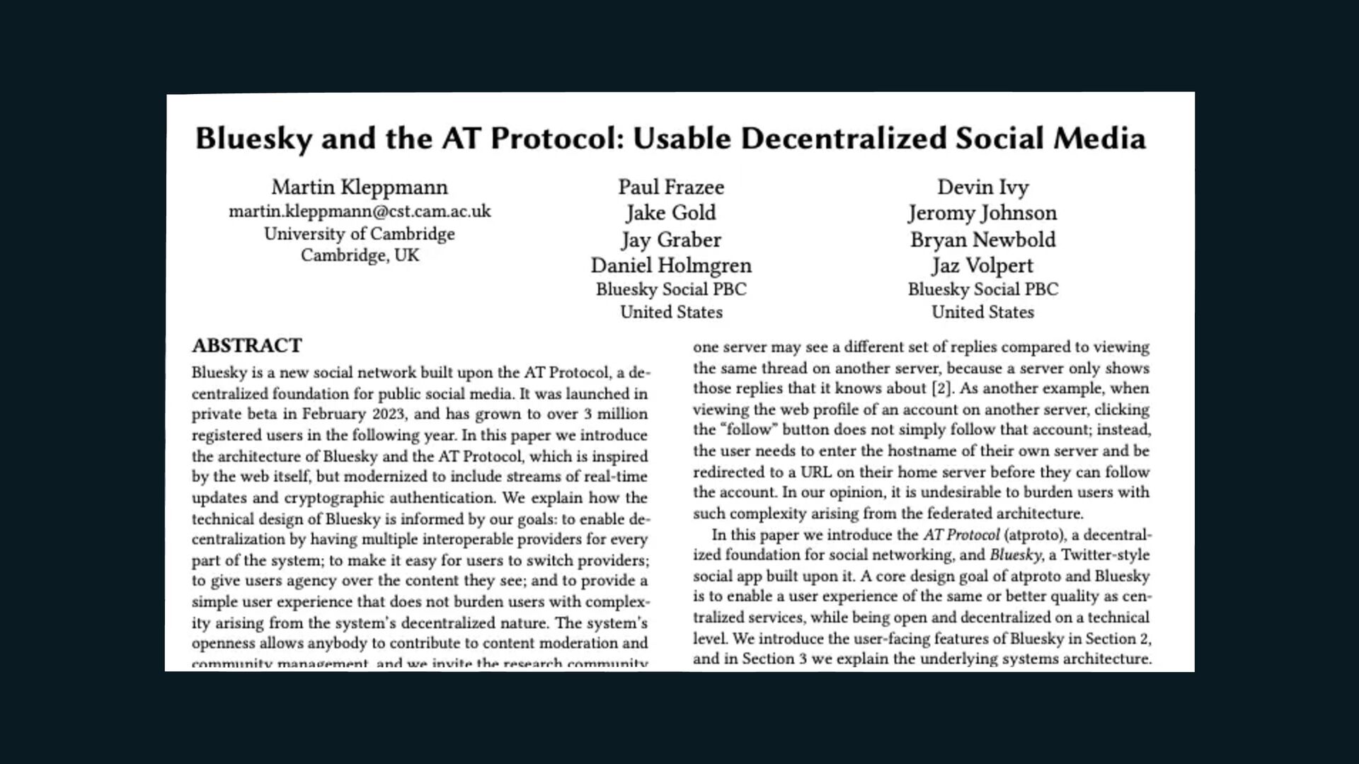
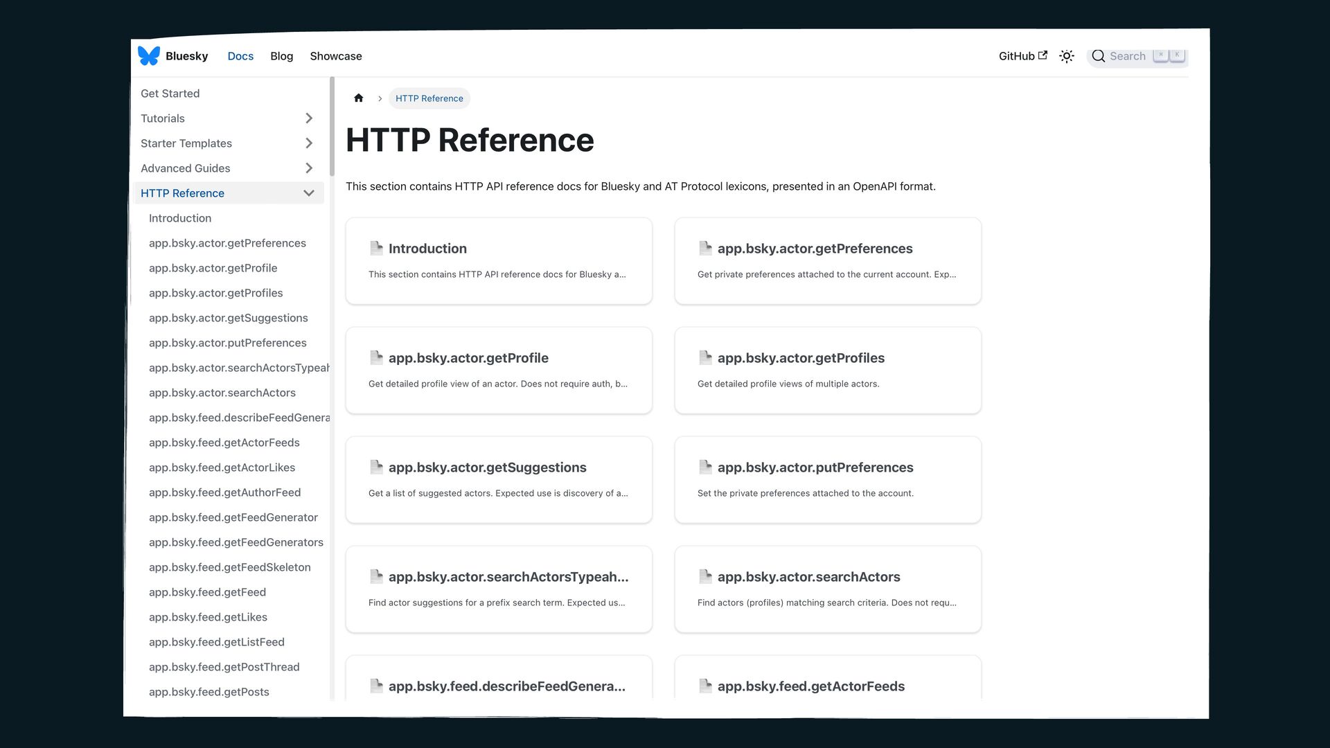
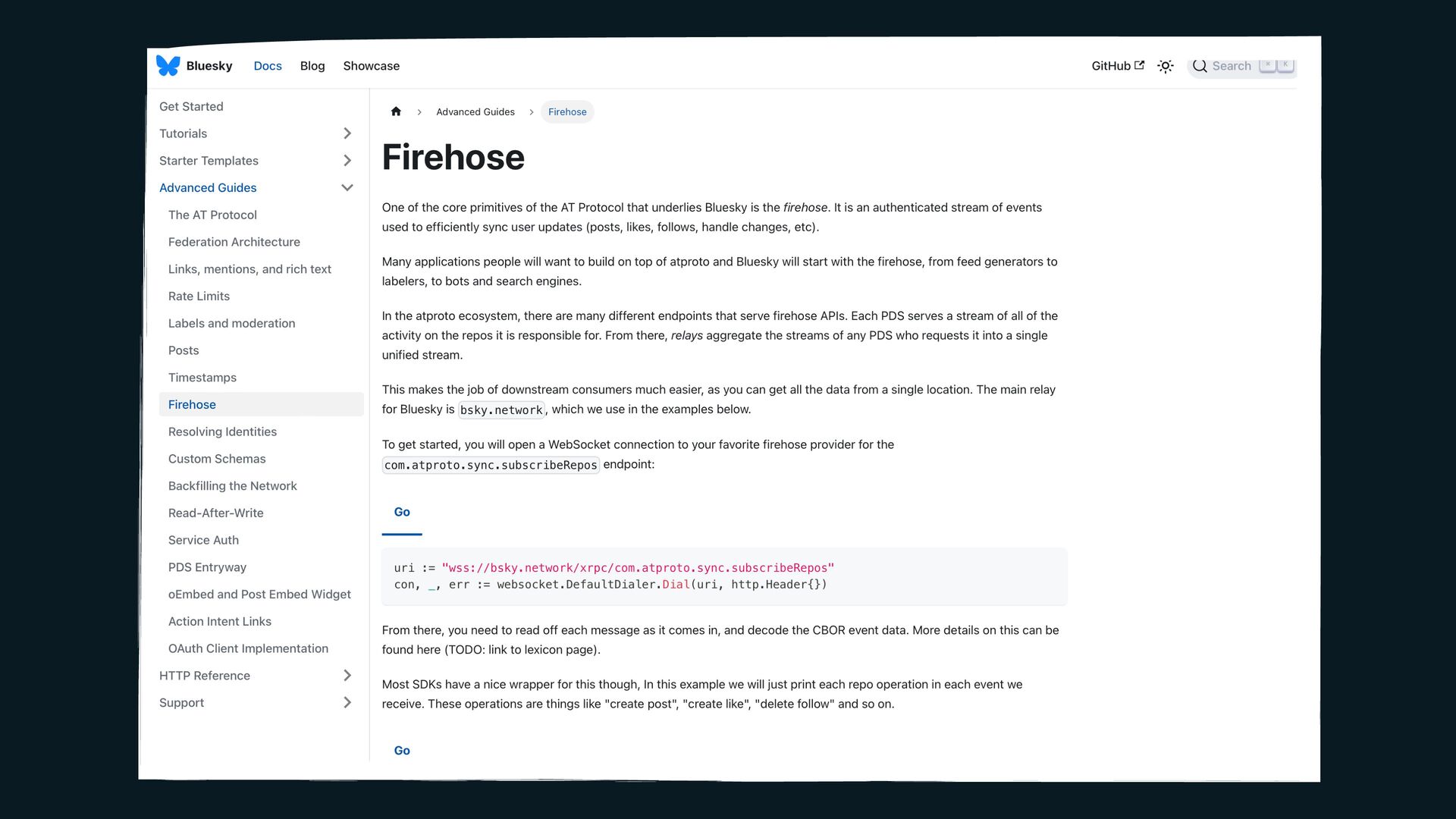
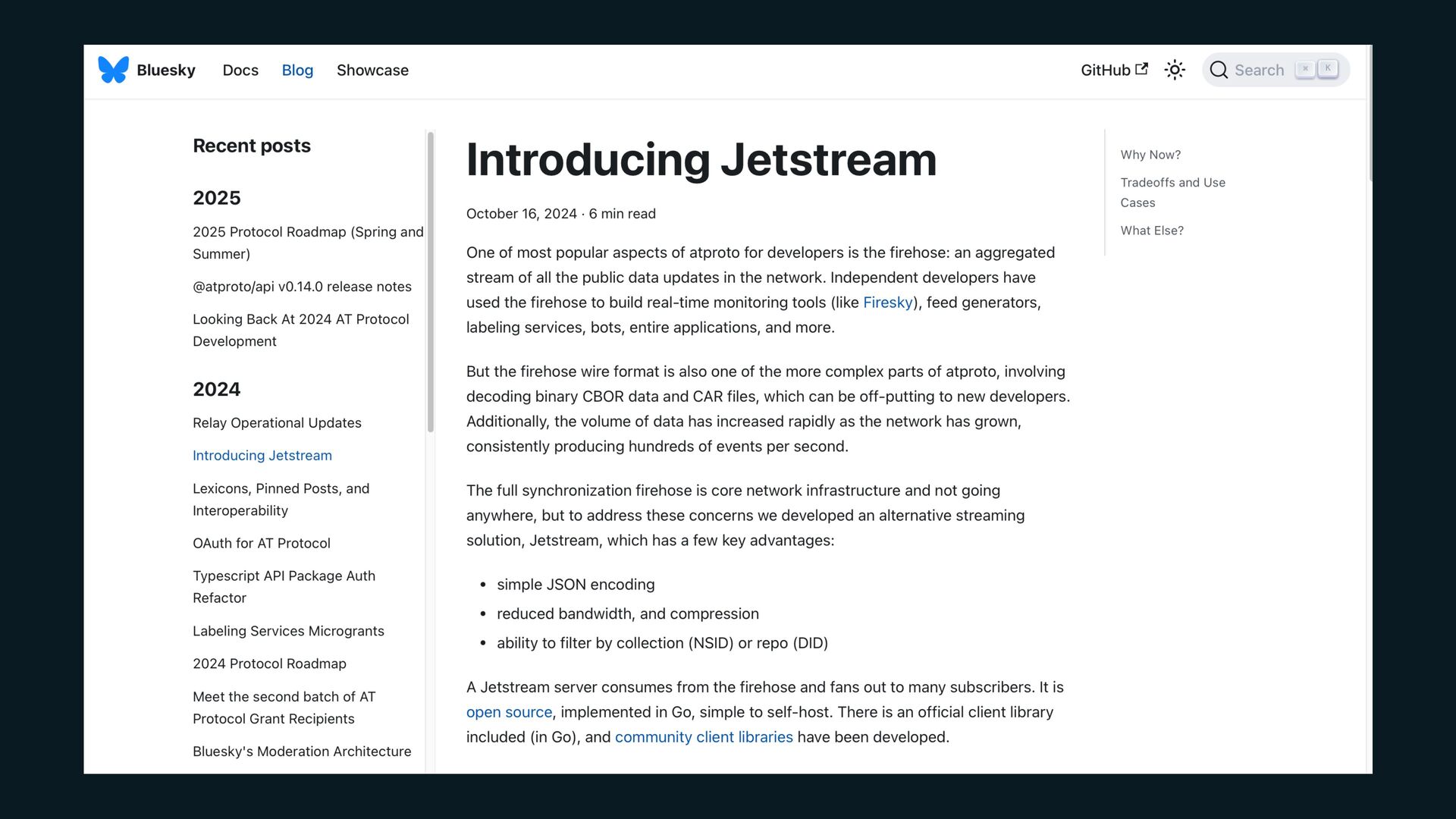
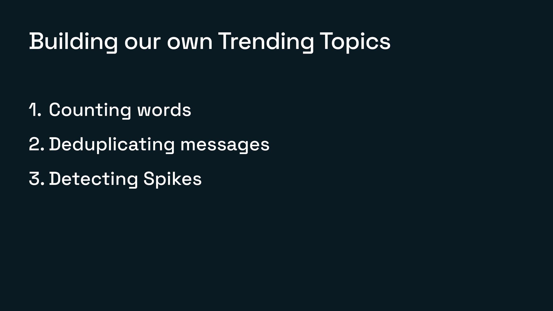
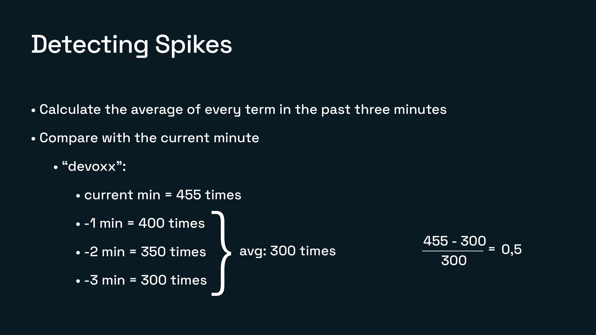
How I used them together to build an efficient version of Trending Topics for Bluesky

By the end, you’ll see how these tools help you process large data streams without blowing up your memory, and how to apply them in real-world systems where being fast matters more than being perfect.

Transcript

1. Count-Min Sketch, Bloom Filter, Top K: Efficient probabilistic data structures Raphael De Lio
2. A little bit of context
5. 31 August • Internet Providers started blocking Twi tt er Timeline
6. 1 September • Bluesky gets 1 million new users Timeline
11. One of many things BSKY doesn’t have… didn’t
12. Blooming Trending Topics on Bluesky
13. Building my own Trending Topics 1. Listen to Bluesky’s JetStream 2. Parse each message and extract individual terms 3. Filter noise 4. Count these terms 5. Sort them by frequency 6. Detect spikes in usage
14. Step 1: Listen to the JetStream
15. Spring Web Socket
16. Step 2: Counting terms
17. Sorted Set
18. Sorted Set • Every minute of data (~22000 terms) is consuming around ~2MB. • I also want to keep historical data so that I can track the spikes of trending topics and further analysis. • This translates to (2 * 60 * 24)MB per day (2.8GB) or ~1TB per year.
19. That’s when I heard of Probabilistic Data Structures Do you know what probabilistic data structures are? No Good for you! You’ll have to prepare a presentation about it! I would prefer not to
20. Deterministic vs Probabilistic • Deterministic structures always give the exact answer. • Probabilistic ones trade some accuracy for speed and space. • Think: HashMap (deterministic) vs Bloom Filter (probabilistic). • Probabilistic is great when “probably correct” is good enough and we’re dealing with huge streams of data.
21. Count-Min Sketch • A probablistic data structure included in Redis 8 • Used to estimate the frequency of elements in a data stream • Operates with space-e ff i ciency, using a fi xed amount of memory regardless of data scale • The advantage of using it is that it may consume way less memory by giving up on accuracy How many times have I been mentioned?
22. How it works…
23. Count-Min Sketch • Internally it’s a grid (sketch) of w (width) and d (depth) • The rows (d) represent the number of hash functions. The columns (w) represent the counter array for each of the hashing functions 0 0 0 0 0 0 0 0 0 0 0 0 0 0 0 fi xed size
24. Count-Min Sketch: Incrementing 0 0 0 0 0 0 0 0 0 0 0 0 0 0 0 Hash1(“redis”) % 5 = 2 Hash2(“redis”) % 5 = 4 Hash3(“redis”) % 5 = 1 CMS.INCRBY terms redis 1 1 1 1 CMS.INCRBY terms redis 1
25. 0 0 0 0 0 0 0 0 0 0 0 0 0 0 0 Hash1(“pets”) % 5 = 0 Hash2(“pets”) % 5 = 3 Hash3(“pets”) % 5 = 1 CMS.INCRBY terms pets 1 1 1 1 1 1 2 Count-Min Sketch: Incrementing CMS.INCRBY terms pets 1
26. 0 0 0 0 0 0 0 0 0 0 0 0 0 0 0 Hash1(“cats”) % 5 = 3 Hash2(“cats”) % 5 = 4 Hash3(“cats”) % 5 = 0 CMS.INCRBY terms cats 1 1 1 1 1 1 2 1 2 1 Count-Min Sketch: Incrementing CMS.INCRBY terms cats 1
27. 0 0 0 0 0 0 0 0 0 0 0 0 0 0 0 Hash1(“dogs”) % 5 = 2 Hash2(“dogs”) % 5 = 1 Hash3(“dogs”) % 5 = 3 CMS.INCRBY terms dogs 1 1 1 1 1 1 2 1 2 1 2 1 1 Count-Min Sketch: Incrementing CMS.INCRBY terms dogs 1
28. Count-Min Sketch: Querying 0 0 0 0 0 0 0 0 0 0 0 0 0 0 0 Hash1(“dogs”) % 5 = 2 Hash2(“dogs”) % 5 = 1 Hash3(“dogs”) % 5 = 3 CMS.QUERY terms dogs 1 1 1 1 1 2 1 2 1 2 1 1 2 1 1 CMS.QUERY terms dogs
29. 0 0 0 0 0 0 0 0 0 0 0 0 0 0 0 Hash1(“redis”) % 5 = 2 Hash2(“redis”) % 5 = 4 Hash3(“redis”) % 5 = 1 CMS.QUERY terms redis 1 1 1 1 1 2 1 2 1 2 1 1 2 1 1 Count-Min Sketch: Querying 2 CMS.QUERY terms redis
30. Count-Min Sketch: Probability • The width determines the error rate. • The depth determines the con fi dence in this error rate. For a Sketch of 5/3: • Error rate: 40% • Con fi dence in this error rate: 99.87% 99.87% of the time, the counter will be within 40% of the true value For a Sketch of 2000/10: • Error rate: 0.1% • Con fi dence in this error rate: 99,99% 99.99% of the time, the counter will be within 0.1% of the true value
31. Count-Min Sketch: Probability • The width determines the error rate. • The depth determines the con fi dence in this error rate. For a Sketch of 5/3: • Error rate: 40% • Con fi dence in this error rate: 99.87% 99.87% of the time, the counter will be within 40% of the true value For a Sketch of 2000/10: • Error rate: 0.1% • Con fi dence in this error rate: 99,99% 99.99% of the time, the counter will be within 0.1% of the true value
32. Count-Min Sketch: Implementation
33. Count-Min Sketch: Implementation
34. Count-Min Sketch: Implementation
35. Count-Min Sketch: Implementation
36. Count-Min Sketch: Implementation
37. Count-Min Sketch: Implementation
38. Count-Min Sketch: Implementation
39. Demo time!
40. Step 3: Filtering stop words
41. Bloom Filter • A probabilistic data structure included in Redis 8. • Used to test whether an element is part of a set. • It operates with high space-e ff i ciency, using a fi xed amount of memory no ma tt er how many items are added. • The advantage is that it can use much less memory than a regular set by allowing occasional false positives.
42. How it works…
43. Bloom Filter • Internally it’s a 1D array. • It also works with multiple hash functions. 0 0 0 0 0 0 0 0 fi xed size
44. Bloom Filter: Adding member Hash1(“I’m”) % 8 = 2 Hash2(“I’m”) % 8 = 4 Hash3(“I’m”) % 8 = 1 BF.ADD stop-words “I’m” 0 0 0 0 0 0 0 0 1 1 1 BF.ADD stop-words “I’m”
45. Bloom Filter: Adding member Hash1(“lol”) % 5 = 0 Hash2(“lol”) % 8 = 3 Hash3(“lol”) % 8 = 1 BF.ADD stop-words “lol” 0 0 0 0 0 0 0 0 1 1 1 1 1 1 BF.ADD stop-words “lol”
46. Bloom Filter: Checking if exists BF.EXISTS stop-words “I’m” 0 0 0 0 0 0 0 0 1 1 1 1 1 1 Hash1(“I’m”) % 8 = 2 Hash2(“I’m”) % 8 = 4 Hash3(“I’m”) % 8 = 1 BF.EXISTS stop-words “I’m”
47. Bloom Filter: Checking if exists BF.EXISTS stop-words “devoxx” 0 0 0 0 0 0 0 0 1 1 1 1 1 1 Hash1(“devoxx”) % 8 = 5 Hash2(“devoxx”) % 8 = 4 Hash3(“devoxx”) % 8 = 1 BF.EXISTS stop-words “devoxx”
48. Bloom Filter: Checking if exists BF.EXISTS stop-words “Brazil” 0 0 0 0 0 0 0 0 1 1 1 1 1 1 Hash1(“Brazil”) % 8 = 3 Hash2(“Brazil”) % 8 = 4 Hash3(“Brazil”) % 8 = 1 BF.EXISTS stop-words “Brazil
49. Bloom Filter: Implementation
50. Bloom Filter: Implementation
51. Bloom Filter: Implementation
52. Bloom Filter: Implementation
53. Demo time!
54. Step 4: Detecting Spikes
55. Top K • A probabilistic data structure included in Redis 8. • Used to track the most frequent items in a stream without storing everything. • It operates with fi xed memory, no ma tt er how much data fl ows through. • The advantage is that it can keep only the top items while using much less memory than a full sorted set, at the cost of approximate results. Step 3: Detecting spikes
56. Top K • It’s a 1D array of K slots • It also works with multiple hash functions • It receives a decay How it works 0 1 2 3 4 decay: 0.9
57. Top K Incrementing counter 0 1 2 3 4 TOPK.INCRBY spiking-now “redis" 1 TOPK.INCRBY spiking-now “redis” 1 Hash(“redis”) % 5 = 1 redis: 1 decay: 0.9
58. Top K Incrementing counter 0 1 2 3 4 TOPK.INCRBY spiking-now “devoxx” 1 TOPK.INCRBY spiking-now “devoxx” 1 Hash(“devoxx”) % 5 = 2 redis: 1 decay: 0.9 devoxx: 1
59. Top K Incrementing counter 0 1 2 3 4 TOPK.INCRBY spiking-now “devoxx” 1 TOPK.INCRBY spiking-now “devoxx” 1 Hash(“devoxx”) % 5 = 2 redis: 1 decay: 0.9 devoxx: 1 devoxx: 2
60. Top K Incrementing counter 0 1 2 3 4 TOPK.INCRBY spiking-now “java” 1 TOPK.INCRBY spiking-now “java” 1 Hash(“java”) % 5 = 2 redis: 1 decay: 0,9 devoxx: 2 devoxx: 1 java: 1 2 * 0,9 = 1,8
61. Top K Incrementing counter 0 1 2 3 4 TOPK.INCRBY spiking-now “java” 1 TOPK.INCRBY spiking-now “java” 1 Hash(“java”) % 5 = 2 redis: 1 decay: 0,9 devoxx: 1 java: 1 1 * 0,9 = 0,9
62. Detecting Spikes • Calculate the average of every term in the past three minutes • Compare with the current minute • “devoxx”: • current min = 455 times • -1 min = 400 times • -2 min = 350 times • -3 min = 300 times avg: 300 times } 455 - 300 300 = 0,5
63. Detecting Spikes: Implementation
64. Detecting Spikes: Implementation
65. Detecting Spikes: Implementation
66. Detecting Spikes: Implementation
67. Detecting Spikes: Implementation
68. Detecting Spikes: Implementation
69. Detecting Spikes: Implementation
70. Demo time!
71. Concluding Memory Comparison of one month of data streamed in buckets of 1 minute Purpose Probabilistic (Approx.) Deterministic (Approx.) Counting words ~2.3GB (Count-Min Sketch) ~87GB (Sorted Sets) Filtering stop terms ~2KB (Bloom Filter) ~59KB (Set) Ranking spikes ~3KB (TopK) ~30MB (Sorted Set) Tracking unique words ~36MB (Set) – Total ~2.34GB ~87GB
73. RAPHAEL DE LIO DEVELOPER ADVOCATE *