Lithium-Ion Battery Hardware-in-the-Loop Simula...

Share
Lithium-Ion Battery Hardware-in-the-Loop Simulation — Emulating Charge and Discharge with a SPICE Model and a Bidirectional Power Supply
This lecture explains how a lithium-ion battery emulator under development at Marutsu can take the place of a physical battery when testing a battery management system (BMS) or charger. A microcontroller runs a SPICE-derived battery model with two RC branches in real time. A bidirectional power supply uses the model to reproduce changes in terminal voltage as the battery’s state of charge and current history evolve. The lecture also explains how the emulator handles power flowing back from the charger.
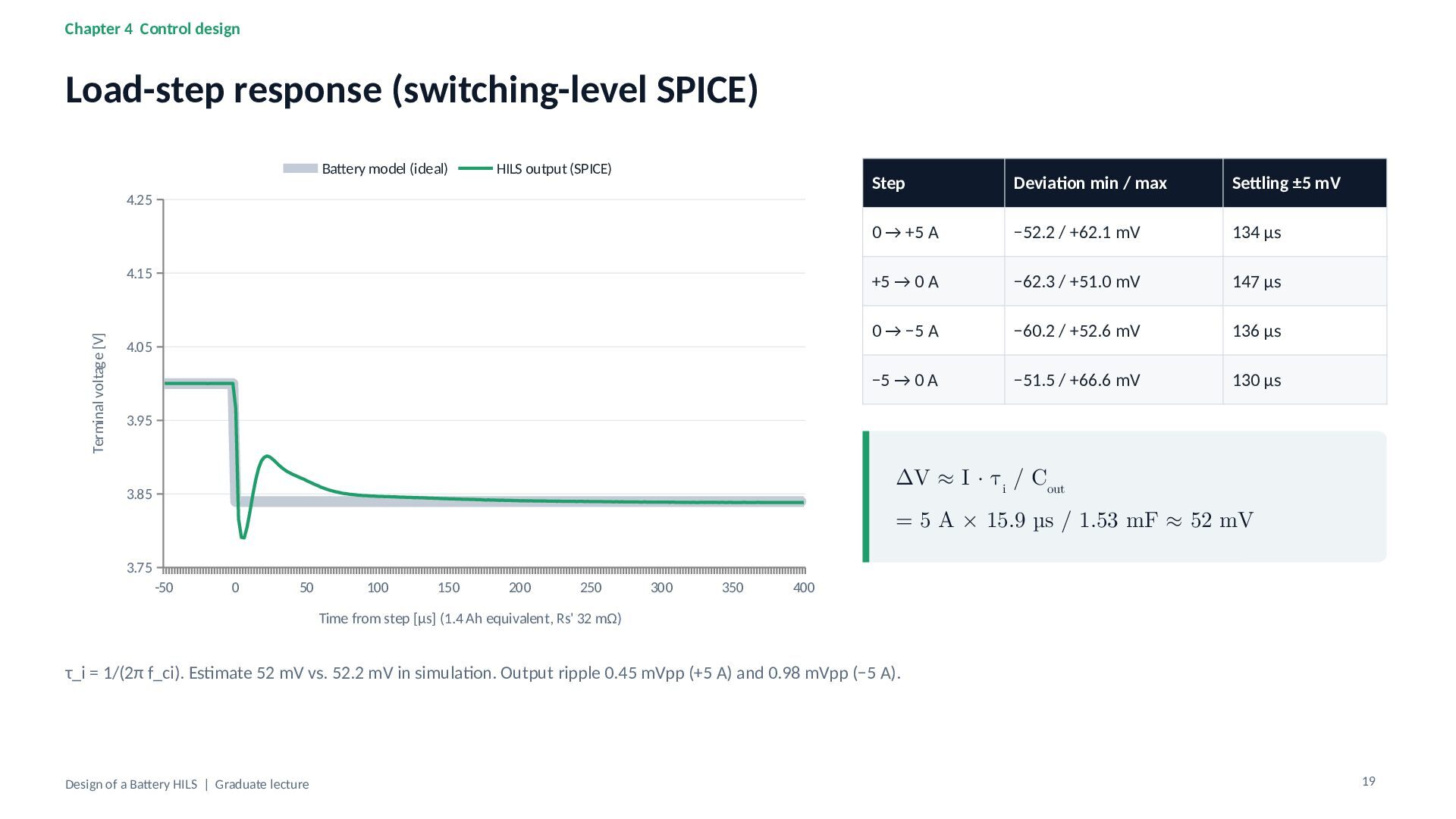
The final section examines a simulated load step from 0 to 5 A. The output voltage settles to within ±5 mV of the model prediction in about 150 µs. The lecture concludes by identifying which aspects of this response still need to be verified on the test bench.

Tsuyoshi Horigome
Transcript
28 slides
-
Design of a Battery HILS From a SPICE battery model
to a real-time battery emulator Graduate lecture (90 min) | Case study: Li-ion battery HILS Rev.A (Marutsuelec Co., Ltd., in development) -
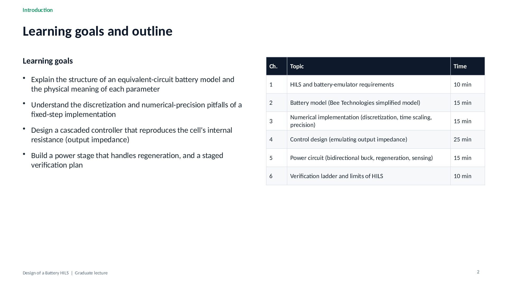
Introduction Learning goals and outline Learning goals • Explain the
structure of an equivalent-circuit battery model and the physical meaning of each parameter • Understand the discretization and numerical-precision pitfalls of a fixed-step implementation • Design a cascaded controller that reproduces the cell's internal resistance (output impedance) • Build a power stage that handles regeneration, and a staged verification plan Design of a Battery HILS | Graduate lecture Ch. Topic Time 1 HILS and battery-emulator requirements 10 min 2 Battery model (Bee Technologies simplified model) 15 min 3 Numerical implementation (discretization, time scaling, precision) 15 min 4 Control design (emulating output impedance) 25 min 5 Power circuit (bidirectional buck, regeneration, sensing) 15 min 6 Verification ladder and limits of HILS 10 min 2 -
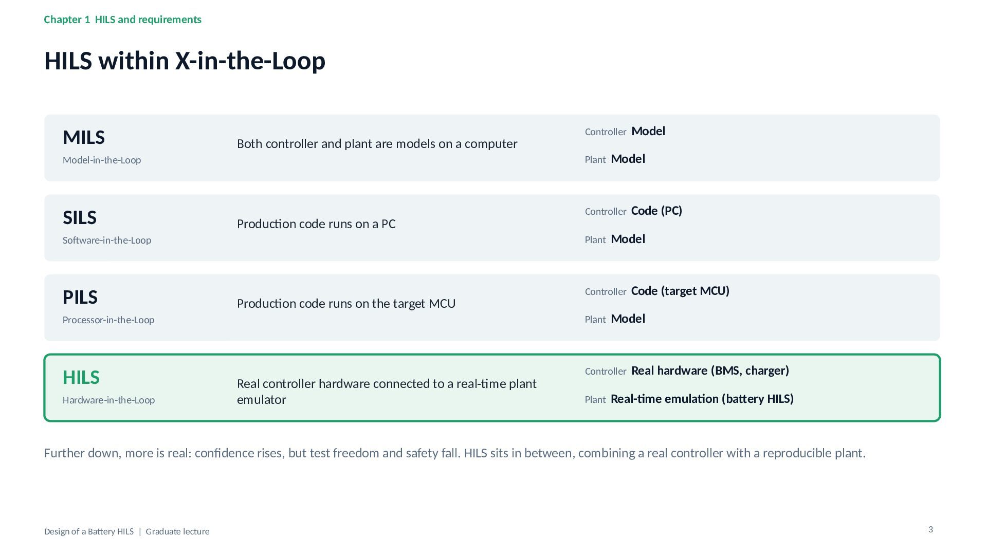
Chapter 1 HILS and requirements HILS within X-in-the-Loop MILS Both
controller and plant are models on a computer Model-in-the-Loop SILS Production code runs on a PC Software-in-the-Loop PILS Production code runs on the target MCU Processor-in-the-Loop HILS Hardware-in-the-Loop Real controller hardware connected to a real-time plant emulator Controller Model Plant Model Controller Code (PC) Plant Model Controller Code (target MCU) Plant Model Controller Real hardware (BMS, charger) Plant Real-time emulation (battery HILS) Further down, more is real: confidence rises, but test freedom and safety fall. HILS sits in between, combining a real controller with a reproducible plant. Design of a Battery HILS | Graduate lecture 3 -
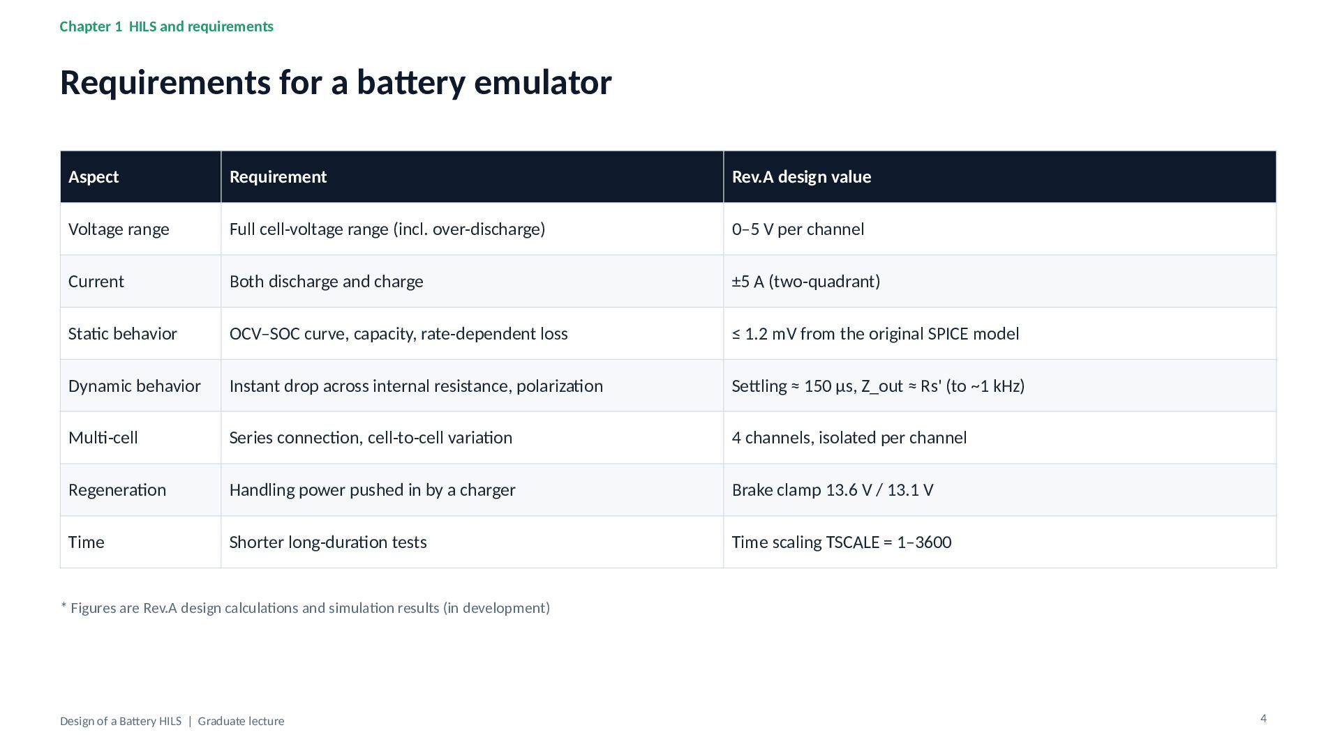
Chapter 1 HILS and requirements Requirements for a battery emulator
Aspect Requirement Rev.A design value Voltage range Full cell-voltage range (incl. over-discharge) 0–5 V per channel Current Both discharge and charge ±5 A (two-quadrant) Static behavior OCV–SOC curve, capacity, rate-dependent loss ≤ 1.2 mV from the original SPICE model Dynamic behavior Instant drop across internal resistance, polarization Settling ≈ 150 µs, Z_out ≈ Rs' (to ~1 kHz) Multi-cell Series connection, cell-to-cell variation 4 channels, isolated per channel Regeneration Handling power pushed in by a charger Brake clamp 13.6 V / 13.1 V Time Shorter long-duration tests Time scaling TSCALE = 1–3600 * Figures are Rev.A design calculations and simulation results (in development) Design of a Battery HILS | Graduate lecture 4 -
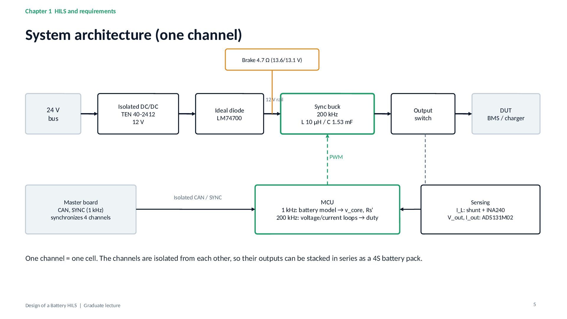
Chapter 1 HILS and requirements System architecture (one channel) Brake
4.7 Ω (13.6/13.1 V) 24 V bus Isolated DC/DC TEN 40-2412 12 V 12 V rail Ideal diode LM74700 Sync buck 200 kHz L 10 µH / C 1.53 mF Output switch DUT BMS / charger PWM Master board CAN, SYNC (1 kHz) synchronizes 4 channels Isolated CAN / SYNC MCU 1 kHz: battery model → v_core, Rs' 200 kHz: voltage/current loops → duty Sensing I_L: shunt + INA240 V_out, I_out: ADS131M02 One channel = one cell. The channels are isolated from each other, so their outputs can be stacked in series as a 4S battery pack. Design of a Battery HILS | Graduate lecture 5 -
Chapter 2 Battery model Equivalent circuit: OCV + series R
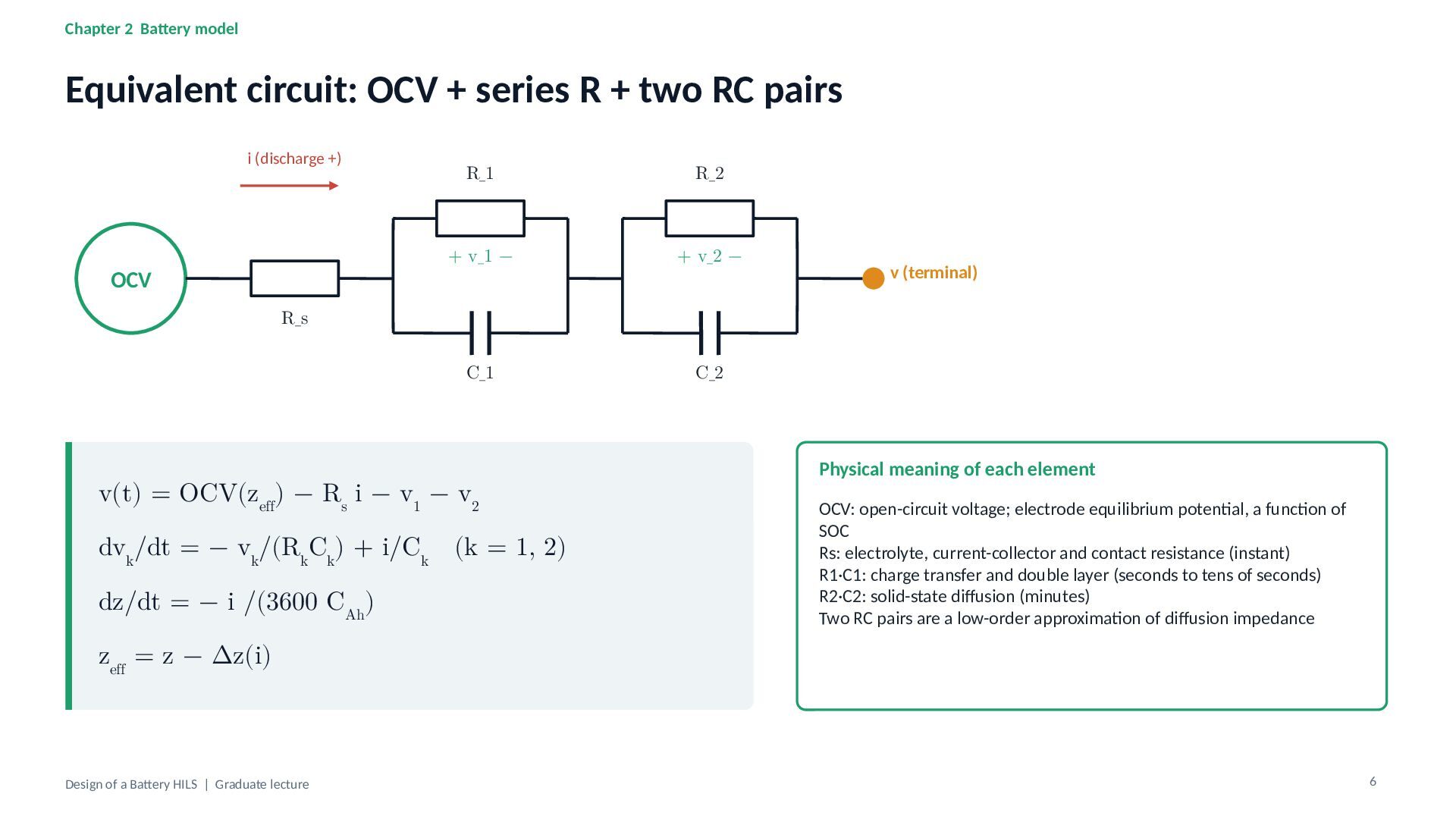
+ two RC pairs i (discharge +) OCV R_1 R_2 + v_1 − + v_2 − C_1 C_2 v (terminal) R_s v(t) = OCV(zeff) − Rs i − v1 − v2 dvk/dt = − vk/(RkCk) + i/Ck (k = 1, 2) dz/dt = − i /(3600 CAh) Physical meaning of each element OCV: open-circuit voltage; electrode equilibrium potential, a function of SOC Rs: electrolyte, current-collector and contact resistance (instant) R1·C1: charge transfer and double layer (seconds to tens of seconds) R2·C2: solid-state diffusion (minutes) Two RC pairs are a low-order approximation of diffusion impedance zeff = z − Δz(i) Design of a Battery HILS | Graduate lecture 6 -
Chapter 2 Battery model Parameters of the Bee Technologies simplified
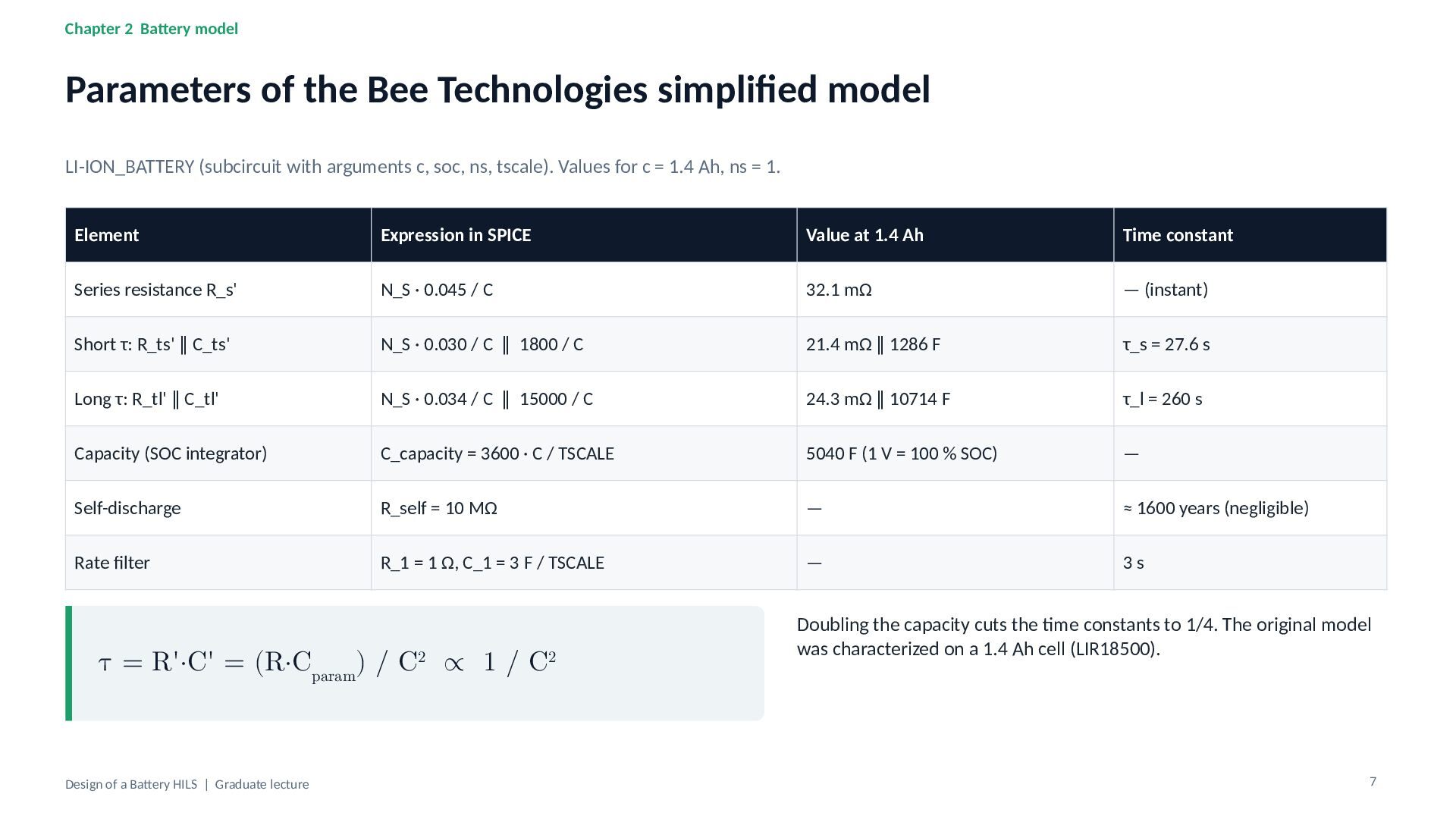
model LI-ION_BATTERY (subcircuit with arguments c, soc, ns, tscale). Values for c = 1.4 Ah, ns = 1. Element Expression in SPICE Value at 1.4 Ah Time constant Series resistance R_s' N_S · 0.045 / C 32.1 mΩ — (instant) Short τ: R_ts' ∥ C_ts' N_S · 0.030 / C ∥ 1800 / C 21.4 mΩ ∥ 1286 F τ_s = 27.6 s Long τ: R_tl' ∥ C_tl' N_S · 0.034 / C ∥ 15000 / C 24.3 mΩ ∥ 10714 F τ_l = 260 s Capacity (SOC integrator) C_capacity = 3600 · C / TSCALE 5040 F (1 V = 100 % SOC) — Self-discharge R_self = 10 MΩ — ≈ 1600 years (negligible) Rate filter R_1 = 1 Ω, C_1 = 3 F / TSCALE — 3s τ = R'·C' = (R·Cparam) / C2 ∝ 1 / C2 Design of a Battery HILS | Graduate lecture Doubling the capacity cuts the time constants to 1/4. The original model was characterized on a 1.4 Ah cell (LIR18500). 7 -
Chapter 2 Battery model OCV–SOC: lookup table + exponential correction
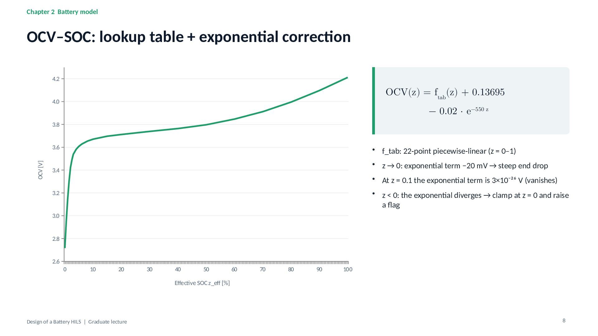
4.2 OCV(z) = ftab(z) + 0.13695 4.0 − 0.02 · e−550 z 3.8 OCV [V] 3.6 • f_tab: 22-point piecewise-linear (z = 0–1) • z → 0: exponential term −20 mV → steep end drop 3.4 • At z = 0.1 the exponential term is 3×10⁻²⁶ V (vanishes) • z < 0: the exponential diverges → clamp at z = 0 and raise a flag 3.2 3.0 2.8 2.6 0 10 20 30 40 50 60 70 80 90 100 Effective SOC z_eff [%] Design of a Battery HILS | Graduate lecture 8 -
Chapter 2 Battery model Rate-dependent capacity loss r=I/C (through a
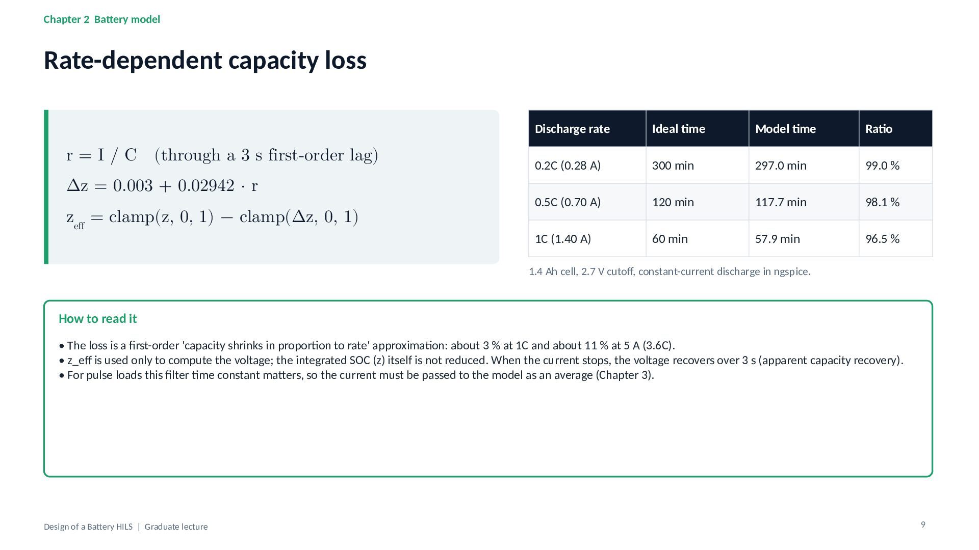
3 s first-order lag) Δz = 0.003 + 0.02942 · r zeff = clamp(z, 0, 1) − clamp(Δz, 0, 1) Discharge rate Ideal time Model time Ratio 0.2C (0.28 A) 300 min 297.0 min 99.0 % 0.5C (0.70 A) 120 min 117.7 min 98.1 % 1C (1.40 A) 60 min 57.9 min 96.5 % 1.4 Ah cell, 2.7 V cutoff, constant-current discharge in ngspice. How to read it • The loss is a first-order 'capacity shrinks in proportion to rate' approximation: about 3 % at 1C and about 11 % at 5 A (3.6C). • z_eff is used only to compute the voltage; the integrated SOC (z) itself is not reduced. When the current stops, the voltage recovers over 3 s (apparent capacity recovery). • For pulse loads this filter time constant matters, so the current must be passed to the model as an average (Chapter 3). Design of a Battery HILS | Graduate lecture 9 -
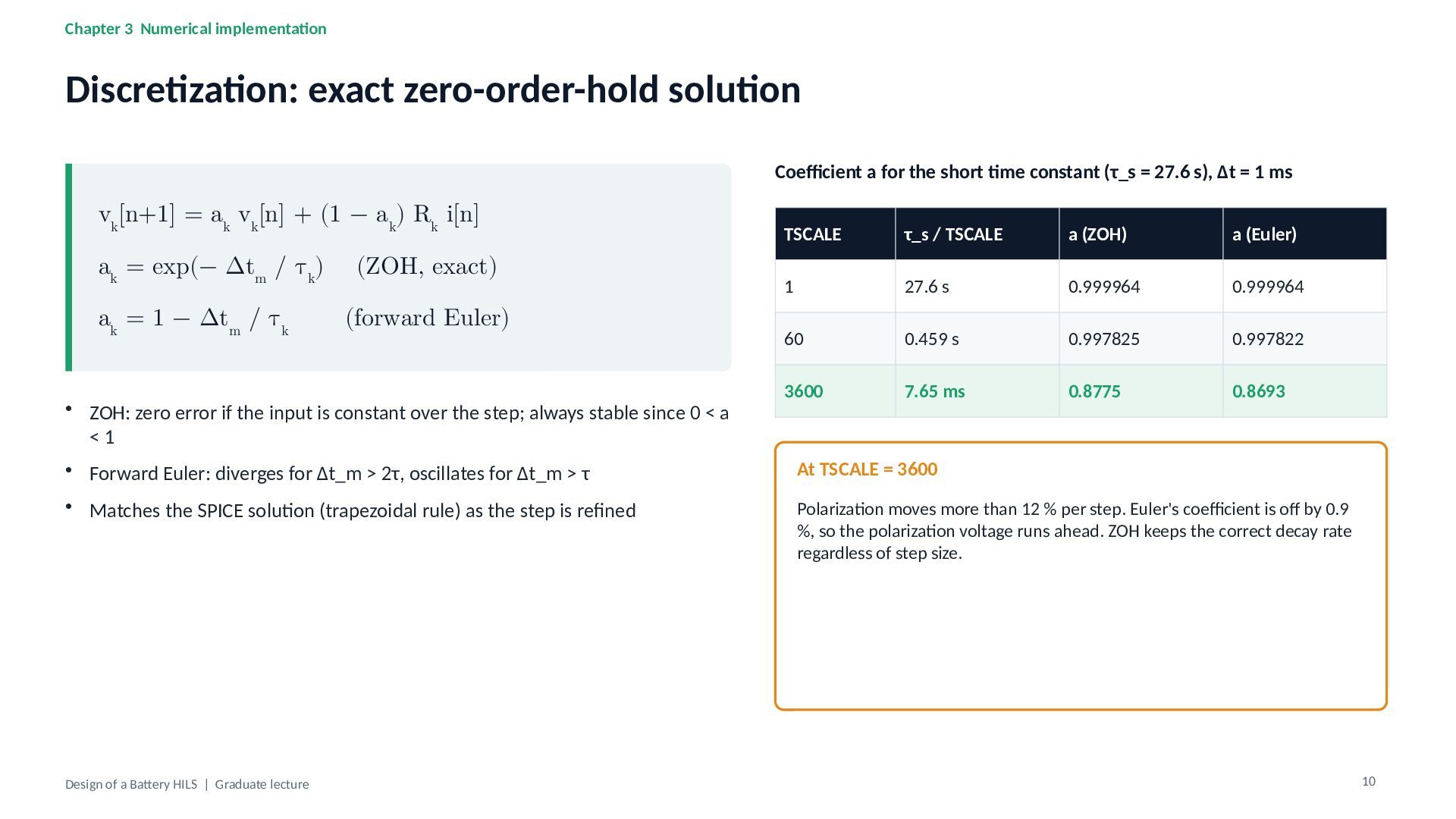
Chapter 3 Numerical implementation Discretization: exact zero-order-hold solution Coefficient a
for the short time constant (τ_s = 27.6 s), Δt = 1 ms vk[n+1] = ak vk[n] + (1 − ak) Rk i[n] ak = exp(− Δtm / τk) (ZOH, exact) ak = 1 − Δtm / τk (forward Euler) • ZOH: zero error if the input is constant over the step; always stable since 0 < a <1 TSCALE τ_s / TSCALE a (ZOH) a (Euler) 1 27.6 s 0.999964 0.999964 60 0.459 s 0.997825 0.997822 3600 7.65 ms 0.8775 0.8693 • Forward Euler: diverges for Δt_m > 2τ, oscillates for Δt_m > τ At TSCALE = 3600 • Matches the SPICE solution (trapezoidal rule) as the step is refined Polarization moves more than 12 % per step. Euler's coefficient is off by 0.9 %, so the polarization voltage runs ahead. ZOH keeps the correct decay rate regardless of step size. Design of a Battery HILS | Graduate lecture 10 -
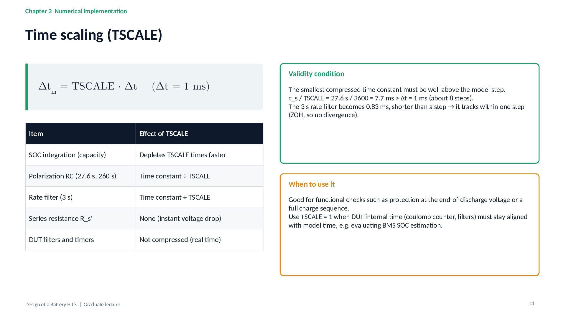
Chapter 3 Numerical implementation Time scaling (TSCALE) Validity condition Δtm
= TSCALE · Δt (Δt = 1 ms) Item Effect of TSCALE SOC integration (capacity) Depletes TSCALE times faster Polarization RC (27.6 s, 260 s) Time constant ÷ TSCALE Rate filter (3 s) Time constant ÷ TSCALE Series resistance R_s' None (instant voltage drop) DUT filters and timers Not compressed (real time) Design of a Battery HILS | Graduate lecture The smallest compressed time constant must be well above the model step. τ_s / TSCALE = 27.6 s / 3600 = 7.7 ms > Δt = 1 ms (about 8 steps). The 3 s rate filter becomes 0.83 ms, shorter than a step → it tracks within one step (ZOH, so no divergence). When to use it Good for functional checks such as protection at the end-of-discharge voltage or a full charge sequence. Use TSCALE = 1 when DUT-internal time (coulomb counter, filters) must stay aligned with model time, e.g. evaluating BMS SOC estimation. 11 -
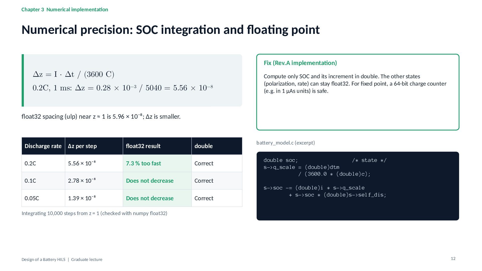
Chapter 3 Numerical implementation Numerical precision: SOC integration and floating
point Fix (Rev.A implementation) Δz = I · Δt / (3600 C) 0.2C, 1 ms: Δz = 0.28 × 10⁻³ / 5040 = 5.56 × 10⁻⁸ Compute only SOC and its increment in double. The other states (polarization, rate) can stay float32. For fixed point, a 64-bit charge counter (e.g. in 1 µAs units) is safe. float32 spacing (ulp) near z ≈ 1 is 5.96 × 10⁻⁸; Δz is smaller. Discharge rate Δz per step float32 result double 0.2C 5.56 × 10⁻⁸ 7.3 % too fast Correct 0.1C 2.78 × 10⁻⁸ Does not decrease Correct 0.05C 1.39 × 10⁻⁸ Does not decrease Correct battery_model.c (excerpt) double soc; /* state */ s->q_scale = (double)dtm / (3600.0 * (double)c); s->soc -= (double)i * s->q_scale + s->soc * (double)s->self_dis; Integrating 10,000 steps from z = 1 (checked with numpy float32) Design of a Battery HILS | Graduate lecture 12 -
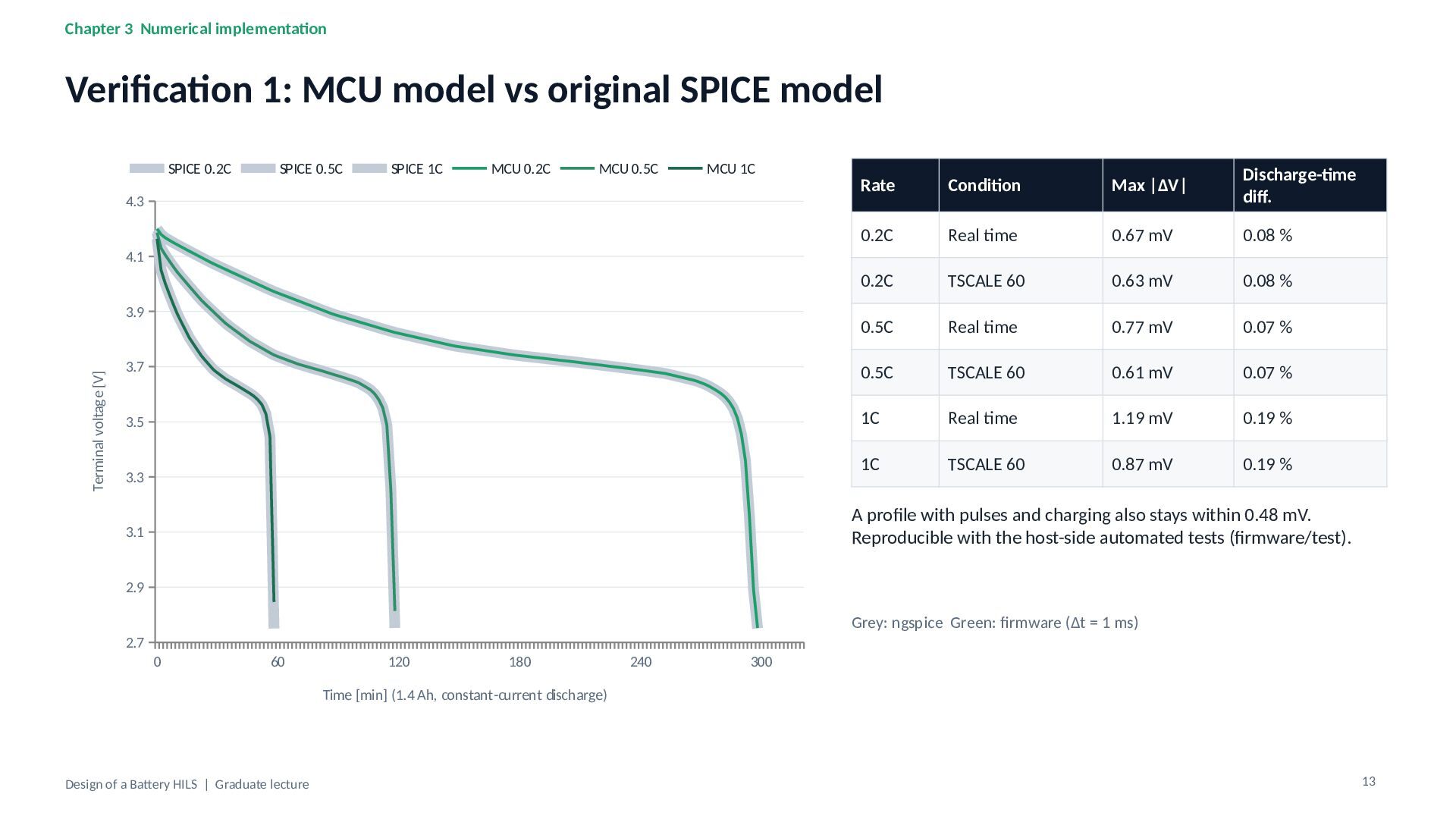
Chapter 3 Numerical implementation Verification 1: MCU model vs original
SPICE model SPICE 0.2C SPICE 0.5C SPICE 1C MCU 0.2C MCU 0.5C MCU 1C Rate Condition Max |ΔV| Discharge-time diff. 0.2C Real time 0.67 mV 0.08 % 0.2C TSCALE 60 0.63 mV 0.08 % 0.5C Real time 0.77 mV 0.07 % 3.7 0.5C TSCALE 60 0.61 mV 0.07 % 3.5 1C Real time 1.19 mV 0.19 % 1C TSCALE 60 0.87 mV 0.19 % 4.3 4.1 Terminal voltage [V] 3.9 3.3 A profile with pulses and charging also stays within 0.48 mV. Reproducible with the host-side automated tests (firmware/test). 3.1 2.9 Grey: ngspice Green: firmware (Δt = 1 ms) 2.7 0 60 120 180 240 300 Time [min] (1.4 Ah, constant-current discharge) Design of a Battery HILS | Graduate lecture 13 -
Chapter 4 Control design Control structure: cascaded control with Rs
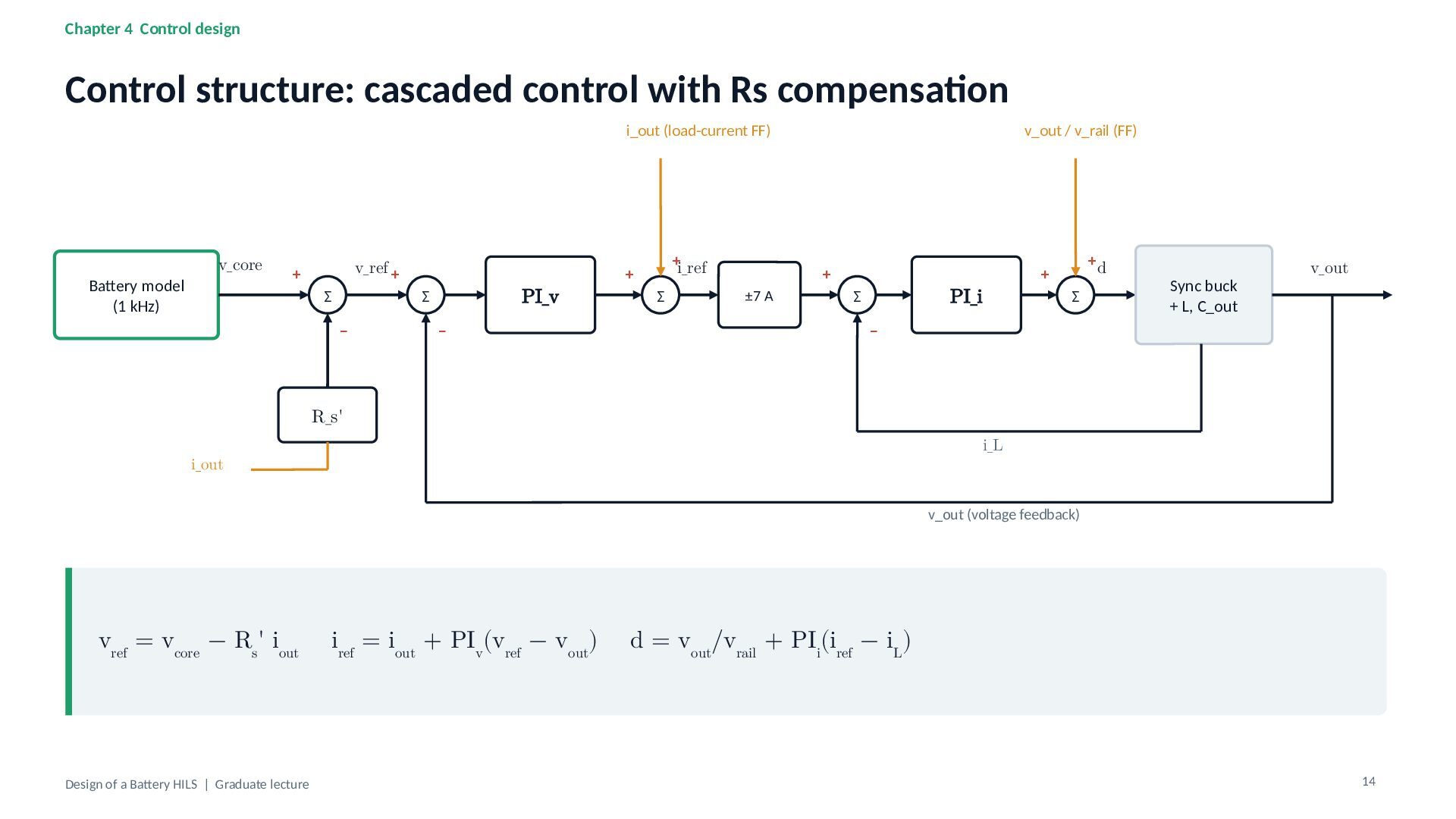
compensation i_out (load-current FF) Battery model (1 kHz) v_core v_ref + + Σ PI_v Σ − − +i_ref + Σ v_out / v_rail (FF) + ±7 A PI_i Σ +d + Σ Sync buck + L, C_out v_out − R_s' i_L i_out v_out (voltage feedback) vref = vcore − Rs' iout Design of a Battery HILS | Graduate lecture iref = iout + PIv(vref − vout) d = vout/vrail + PIi(iref − iL) 14 -
Chapter 4 Control design Creating the output impedance Zout(s) =
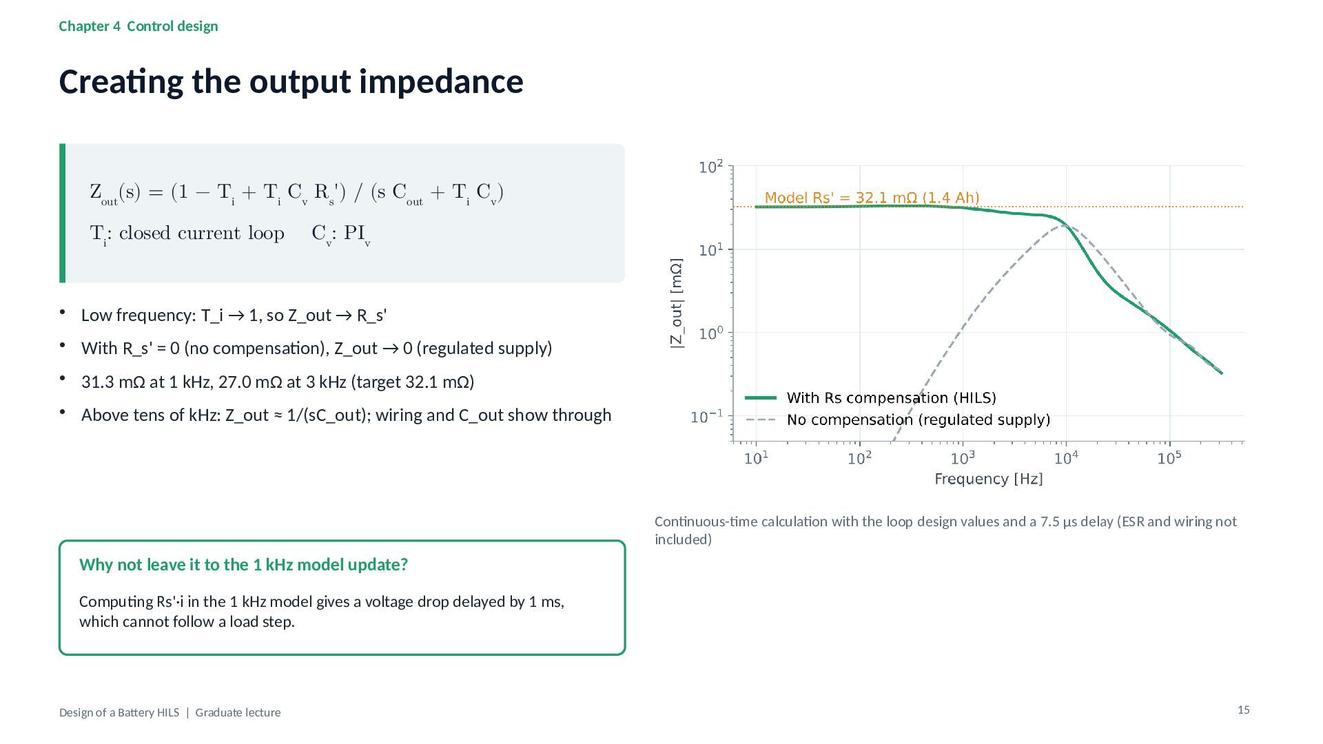
(1 − Ti + Ti Cv Rs') / (s Cout + Ti Cv) Ti: closed current loop Cv: PIv • Low frequency: T_i → 1, so Z_out → R_s' • With R_s' = 0 (no compensation), Z_out → 0 (regulated supply) • 31.3 mΩ at 1 kHz, 27.0 mΩ at 3 kHz (target 32.1 mΩ) • Above tens of kHz: Z_out ≈ 1/(sC_out); wiring and C_out show through Continuous-time calculation with the loop design values and a 7.5 µs delay (ESR and wiring not included) Why not leave it to the 1 kHz model update? Computing Rs'·i in the 1 kHz model gives a voltage drop delayed by 1 ms, which cannot follow a load step. Design of a Battery HILS | Graduate lecture 15 -
Chapter 4 Control design Current-loop design Gi(s) = Vrail /
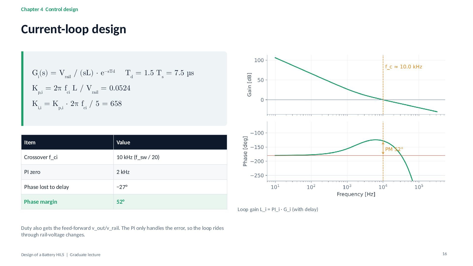
(sL) · e−sTd Td = 1.5 Ts = 7.5 µs Kp,i = 2π fci L / Vrail = 0.0524 Ki,i = Kp,i · 2π fci / 5 = 658 Item Value Crossover f_ci 10 kHz (f_sw / 20) PI zero 2 kHz Phase lost to delay −27° Phase margin 52° Loop gain L_i = PI_i · G_i (with delay) Duty also gets the feed-forward v_out/v_rail. The PI only handles the error, so the loop rides through rail-voltage changes. Design of a Battery HILS | Graduate lecture 16 -
Chapter 4 Control design Voltage-loop design Gv(s) ≈ Ti(s) /
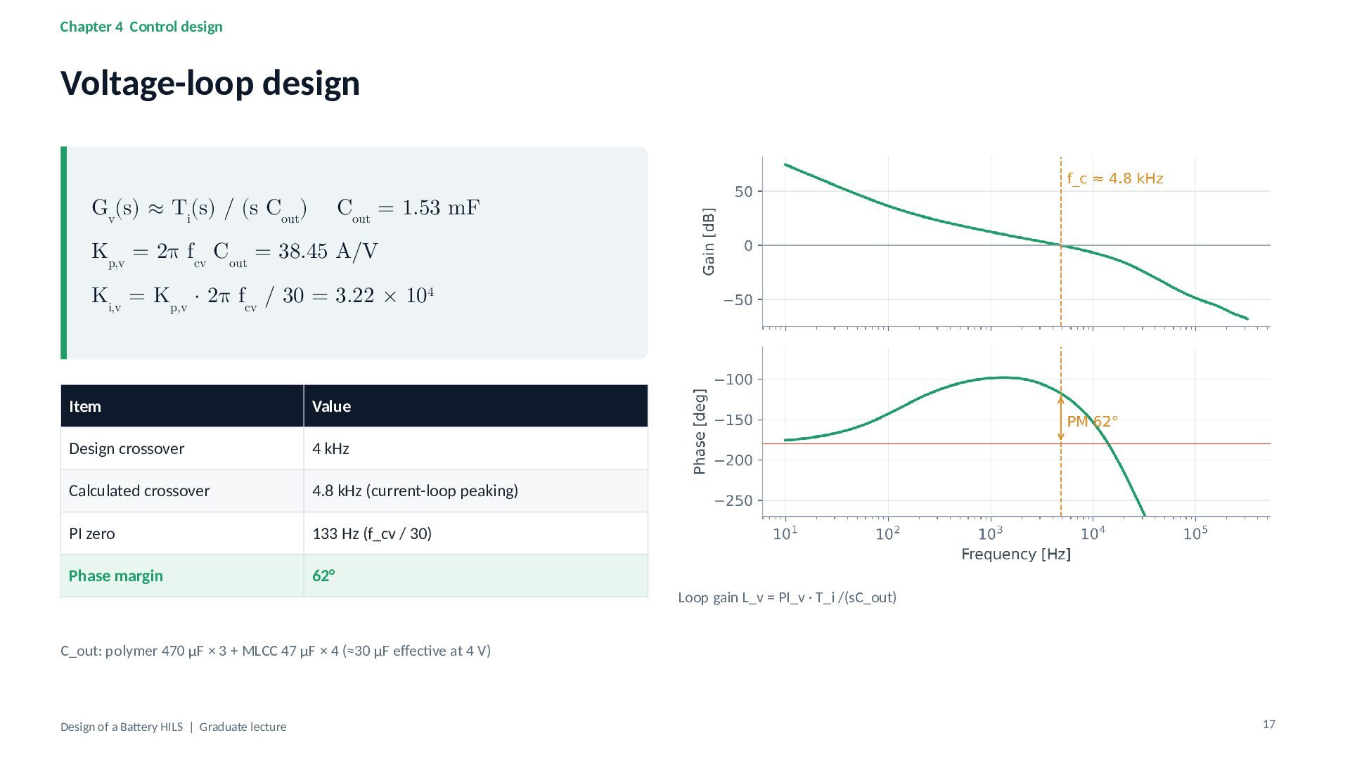
(s Cout) Cout = 1.53 mF Kp,v = 2π fcv Cout = 38.45 A/V Ki,v = Kp,v · 2π fcv / 30 = 3.22 × 10⁴ Item Value Design crossover 4 kHz Calculated crossover 4.8 kHz (current-loop peaking) PI zero 133 Hz (f_cv / 30) Phase margin 62° Loop gain L_v = PI_v · T_i /(sC_out) C_out: polymer 470 µF × 3 + MLCC 47 µF × 4 (≈30 µF effective at 4 V) Design of a Battery HILS | Graduate lecture 17 -
Chapter 4 Control design Implementation details (cell_control.c) /* 200 kHz
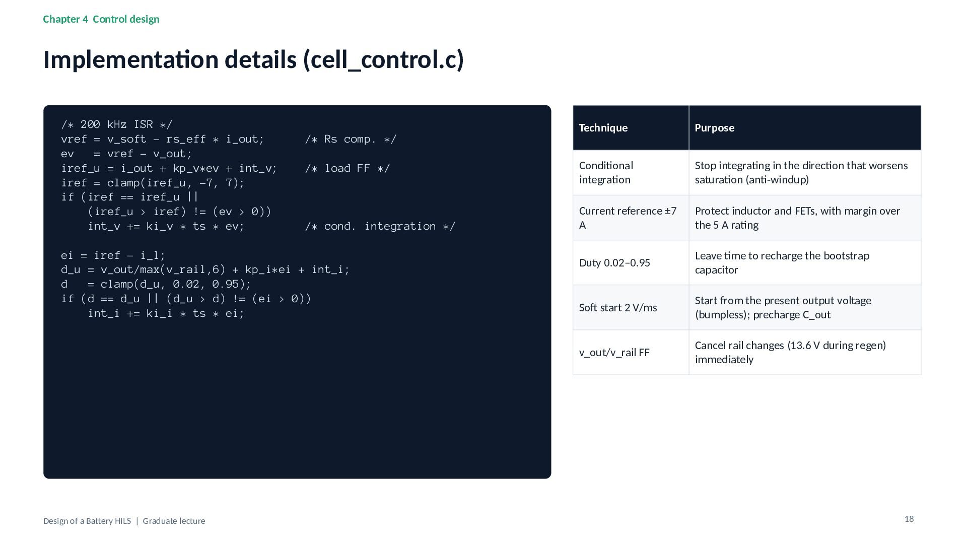
ISR */ vref = v_soft - rs_eff * i_out; ev = vref - v_out; iref_u = i_out + kp_v*ev + int_v; iref = clamp(iref_u, -7, 7); if (iref == iref_u || (iref_u > iref) != (ev > 0)) int_v += ki_v * ts * ev; /* Rs comp. */ /* load FF */ /* cond. integration */ ei = iref - i_l; d_u = v_out/max(v_rail,6) + kp_i*ei + int_i; d = clamp(d_u, 0.02, 0.95); if (d == d_u || (d_u > d) != (ei > 0)) int_i += ki_i * ts * ei; Design of a Battery HILS | Graduate lecture Technique Purpose Conditional integration Stop integrating in the direction that worsens saturation (anti-windup) Current reference ±7 A Protect inductor and FETs, with margin over the 5 A rating Duty 0.02–0.95 Leave time to recharge the bootstrap capacitor Soft start 2 V/ms Start from the present output voltage (bumpless); precharge C_out v_out/v_rail FF Cancel rail changes (13.6 V during regen) immediately 18 -
Chapter 4 Control design Load-step response (switching-level SPICE) Battery model
(ideal) HILS output (SPICE) 4.25 Terminal voltage [V] 4.15 4.05 Step Deviation min / max Settling ±5 mV 0 → +5 A −52.2 / +62.1 mV 134 µs +5 → 0 A −62.3 / +51.0 mV 147 µs 0 → −5 A −60.2 / +52.6 mV 136 µs −5 → 0 A −51.5 / +66.6 mV 130 µs 3.95 ΔV ≈ I · τi / Cout 3.85 = 5 A × 15.9 µs / 1.53 mF ≈ 52 mV 3.75 -50 0 50 100 150 200 250 300 350 400 Time from step [µs] (1.4 Ah equivalent, Rs' 32 mΩ) τ_i = 1/(2π f_ci). Estimate 52 mV vs. 52.2 mV in simulation. Output ripple 0.45 mVpp (+5 A) and 0.98 mVpp (−5 A). Design of a Battery HILS | Graduate lecture 19 -
Chapter 5 Power circuit Bidirectional synchronous buck converter V_rail 12
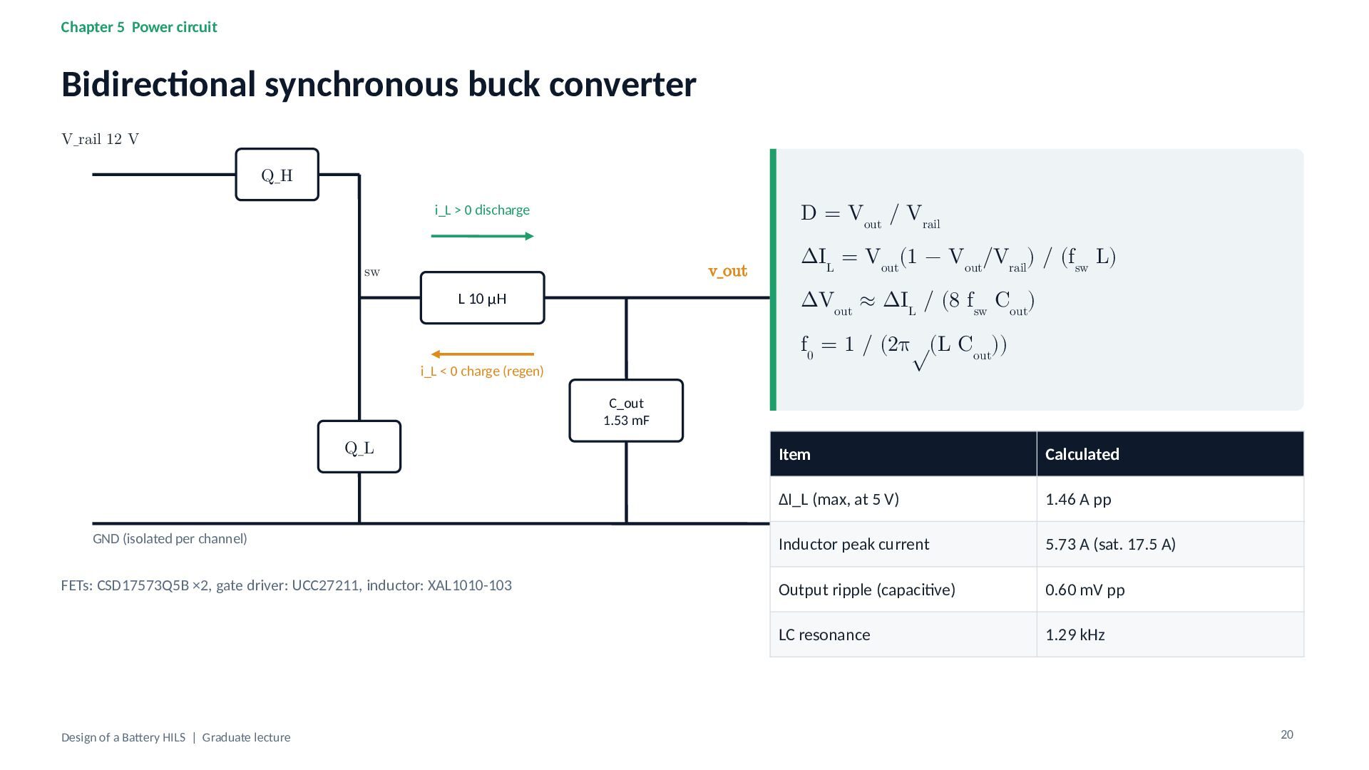
V Q_H D = Vout / Vrail i_L > 0 discharge v_out sw ΔIL = Vout(1 − Vout/Vrail) / (fsw L) ΔVout ≈ ΔIL / (8 fsw Cout) L 10 µH f0 = 1 / (2π√(L Cout)) i_L < 0 charge (regen) C_out 1.53 mF Q_L GND (isolated per channel) FETs: CSD17573Q5B ×2, gate driver: UCC27211, inductor: XAL1010-103 Design of a Battery HILS | Graduate lecture Item Calculated ΔI_L (max, at 5 V) 1.46 A pp Inductor peak current 5.73 A (sat. 17.5 A) Output ripple (capacitive) 0.60 mV pp LC resonance 1.29 kHz 20 -
Chapter 5 Power circuit Losses and supply sizing Loss breakdown
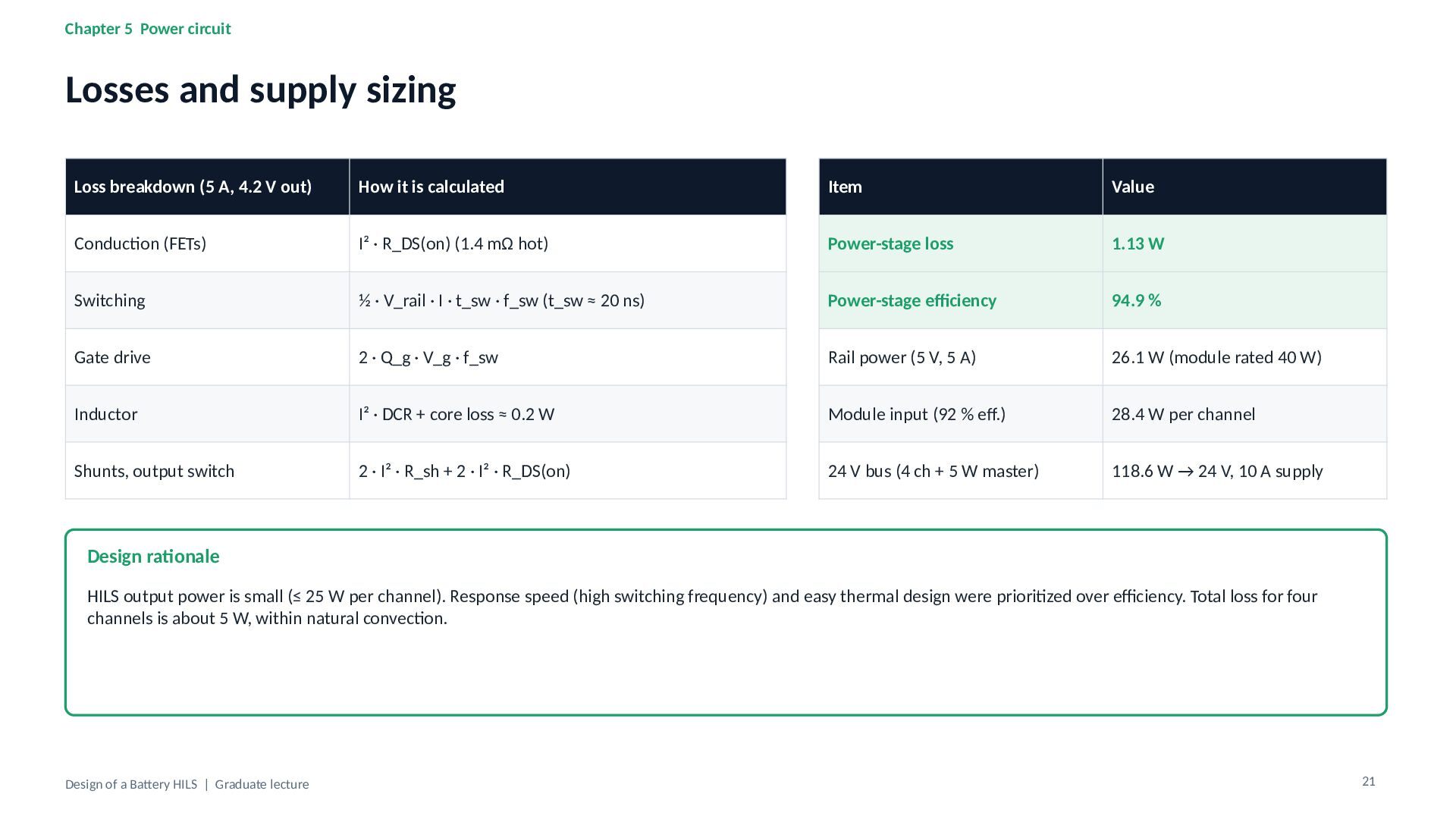
(5 A, 4.2 V out) How it is calculated Item Value Conduction (FETs) I² · R_DS(on) (1.4 mΩ hot) Power-stage loss 1.13 W Switching ½ · V_rail · I · t_sw · f_sw (t_sw ≈ 20 ns) Power-stage efficiency 94.9 % Gate drive 2 · Q_g · V_g · f_sw Rail power (5 V, 5 A) 26.1 W (module rated 40 W) Inductor I² · DCR + core loss ≈ 0.2 W Module input (92 % eff.) 28.4 W per channel Shunts, output switch 2 · I² · R_sh + 2 · I² · R_DS(on) 24 V bus (4 ch + 5 W master) 118.6 W → 24 V, 10 A supply Design rationale HILS output power is small (≤ 25 W per channel). Response speed (high switching frequency) and easy thermal design were prioritized over efficiency. Total loss for four channels is about 5 W, within natural convection. Design of a Battery HILS | Graduate lecture 21 -
Chapter 5 Power circuit Handling regenerated energy Pregen = Vout
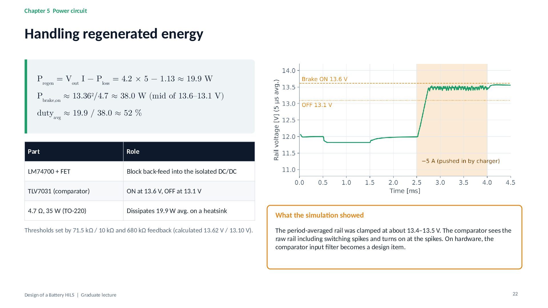
I − Ploss = 4.2 × 5 − 1.13 ≈ 19.9 W Pbrake,on ≈ 13.362/4.7 ≈ 38.0 W (mid of 13.6–13.1 V) dutyavg ≈ 19.9 / 38.0 ≈ 52 % Part Role LM74700 + FET Block back-feed into the isolated DC/DC TLV7031 (comparator) ON at 13.6 V, OFF at 13.1 V 4.7 Ω, 35 W (TO-220) Dissipates 19.9 W avg. on a heatsink Thresholds set by 71.5 kΩ / 10 kΩ and 680 kΩ feedback (calculated 13.62 V / 13.10 V). Design of a Battery HILS | Graduate lecture What the simulation showed The period-averaged rail was clamped at about 13.4–13.5 V. The comparator sees the raw rail including switching spikes and turns on at the spikes. On hardware, the comparator input filter becomes a design item. 22 -
Chapter 5 Power circuit Sensing and isolation Signal Sensor Gain
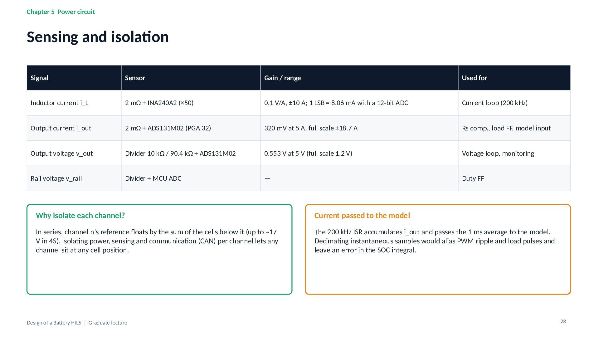
/ range Used for Inductor current i_L 2 mΩ + INA240A2 (×50) 0.1 V/A, ±10 A; 1 LSB = 8.06 mA with a 12-bit ADC Current loop (200 kHz) Output current i_out 2 mΩ + ADS131M02 (PGA 32) 320 mV at 5 A, full scale ±18.7 A Rs comp., load FF, model input Output voltage v_out Divider 10 kΩ / 90.4 kΩ + ADS131M02 0.553 V at 5 V (full scale 1.2 V) Voltage loop, monitoring Rail voltage v_rail Divider + MCU ADC — Duty FF Why isolate each channel? Current passed to the model In series, channel n's reference floats by the sum of the cells below it (up to ~17 V in 4S). Isolating power, sensing and communication (CAN) per channel lets any channel sit at any cell position. The 200 kHz ISR accumulates i_out and passes the 1 ms average to the model. Decimating instantaneous samples would alias PWM ripple and load pulses and leave an error in the SOC integral. Design of a Battery HILS | Graduate lecture 23 -
Chapter 6 Verification and limits of HILS Verification ladder 1
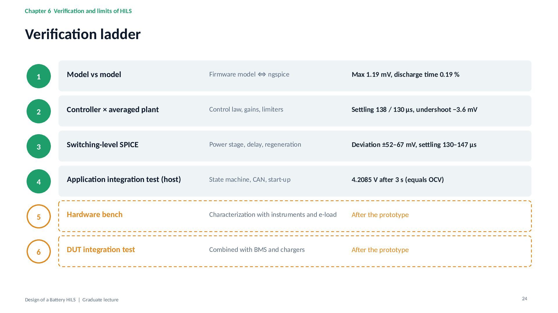
Model vs model Firmware model ⇔ ngspice Max 1.19 mV, discharge time 0.19 % 2 Controller × averaged plant Control law, gains, limiters Settling 138 / 130 µs, undershoot −3.6 mV 3 Switching-level SPICE Power stage, delay, regeneration Deviation ±52–67 mV, settling 130–147 µs 4 Application integration test (host) State machine, CAN, start-up 4.2085 V after 3 s (equals OCV) 5 Hardware bench Characterization with instruments and e-load After the prototype 6 DUT integration test Combined with BMS and chargers After the prototype Design of a Battery HILS | Graduate lecture 24 -
Chapter 6 Verification and limits of HILS Limits and caveats
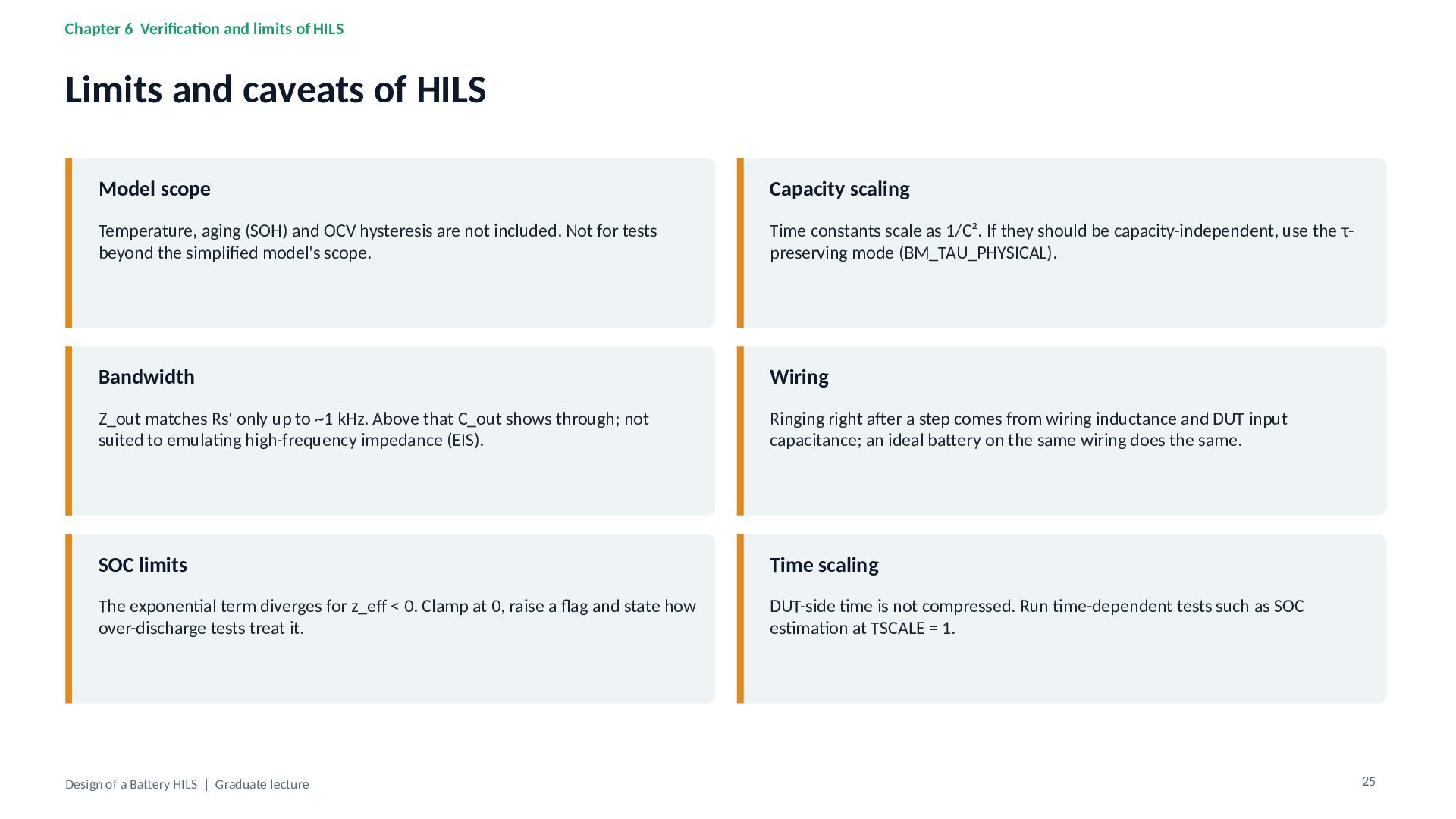
of HILS Model scope Capacity scaling Temperature, aging (SOH) and OCV hysteresis are not included. Not for tests beyond the simplified model's scope. Time constants scale as 1/C². If they should be capacity-independent, use the τpreserving mode (BM_TAU_PHYSICAL). Bandwidth Wiring Z_out matches Rs' only up to ~1 kHz. Above that C_out shows through; not suited to emulating high-frequency impedance (EIS). Ringing right after a step comes from wiring inductance and DUT input capacitance; an ideal battery on the same wiring does the same. SOC limits Time scaling The exponential term diverges for z_eff < 0. Clamp at 0, raise a flag and state how over-discharge tests treat it. DUT-side time is not compressed. Run time-dependent tests such as SOC estimation at TSCALE = 1. Design of a Battery HILS | Graduate lecture 25 -
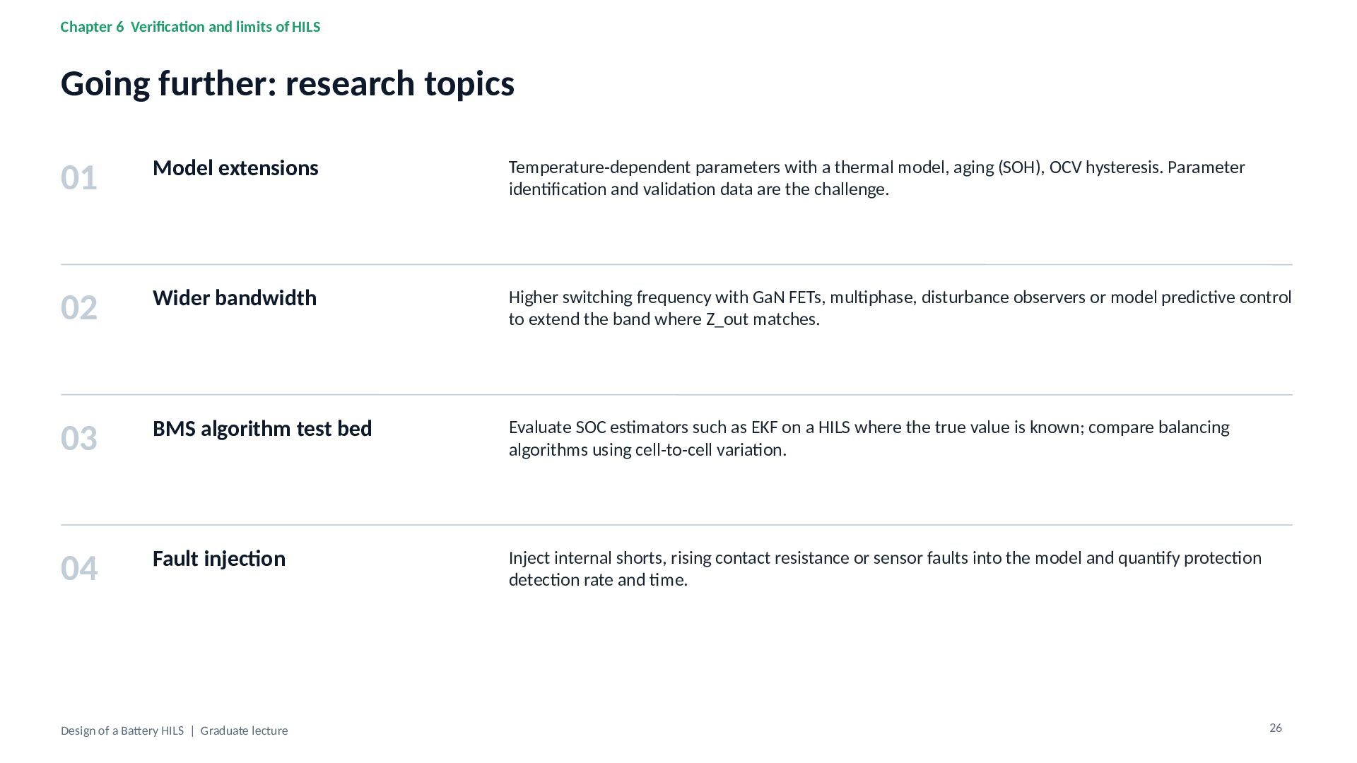
Chapter 6 Verification and limits of HILS Going further: research
topics 01 Model extensions Temperature-dependent parameters with a thermal model, aging (SOH), OCV hysteresis. Parameter identification and validation data are the challenge. 02 Wider bandwidth Higher switching frequency with GaN FETs, multiphase, disturbance observers or model predictive control to extend the band where Z_out matches. 03 BMS algorithm test bed Evaluate SOC estimators such as EKF on a HILS where the true value is known; compare balancing algorithms using cell-to-cell variation. 04 Fault injection Inject internal shorts, rising contact resistance or sensor faults into the model and quantify protection detection rate and time. Design of a Battery HILS | Graduate lecture 26 -
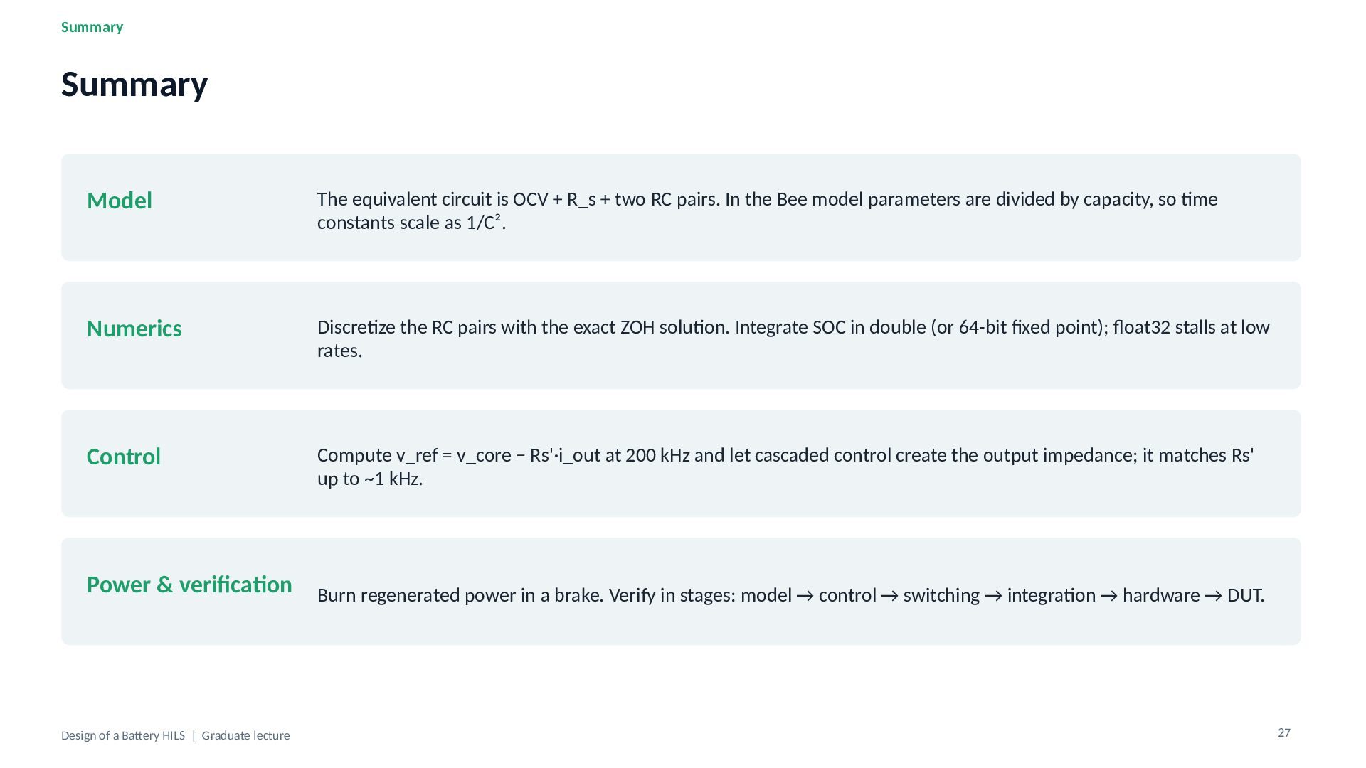
Summary Summary Model The equivalent circuit is OCV + R_s
+ two RC pairs. In the Bee model parameters are divided by capacity, so time constants scale as 1/C². Numerics Discretize the RC pairs with the exact ZOH solution. Integrate SOC in double (or 64-bit fixed point); float32 stalls at low rates. Control Compute v_ref = v_core − Rs'·i_out at 200 kHz and let cascaded control create the output impedance; it matches Rs' up to ~1 kHz. Power & verification Design of a Battery HILS | Graduate lecture Burn regenerated power in a brake. Verify in stages: model → control → switching → integration → hardware → DUT. 27 -
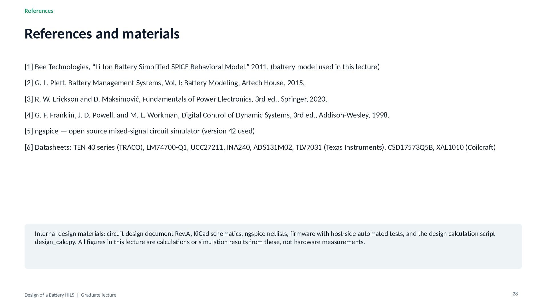
References References and materials [1] Bee Technologies, “Li-Ion Battery Simplified
SPICE Behavioral Model,” 2011. (battery model used in this lecture) [2] G. L. Plett, Battery Management Systems, Vol. I: Battery Modeling, Artech House, 2015. [3] R. W. Erickson and D. Maksimović, Fundamentals of Power Electronics, 3rd ed., Springer, 2020. [4] G. F. Franklin, J. D. Powell, and M. L. Workman, Digital Control of Dynamic Systems, 3rd ed., Addison-Wesley, 1998. [5] ngspice — open source mixed-signal circuit simulator (version 42 used) [6] Datasheets: TEN 40 series (TRACO), LM74700-Q1, UCC27211, INA240, ADS131M02, TLV7031 (Texas Instruments), CSD17573Q5B, XAL1010 (Coilcraft) Internal design materials: circuit design document Rev.A, KiCad schematics, ngspice netlists, firmware with host-side automated tests, and the design calculation script design_calc.py. All figures in this lecture are calculations or simulation results from these, not hardware measurements. Design of a Battery HILS | Graduate lecture 28
 beetech
 shift_evolve
 jacopen
 silmin_
 ota1022
 swdtkuy
 dkduppf
 110y
 endonanana
 minorun365
 yappli_developers
 harutiro
 tomoki10
 emna__ayadi
 andyhume
 aleyda
 kneath
 csswizardry
 rkaga
 ipullrank
 tonyrice
 palkan
 khoart
 davidcarrasco
 jonoalderson