Introduction to Jupyter Notebooks & Data Analytics with Kaggle

Workshop given on Pyladies Dublin

Transcript

1. Introduction to Jupyter Notebooks & Data Analysis using Kaggle
2. LETICIA PORTELLA /in/leportella @leportella @leleportella leportella.com pizzadedados.com
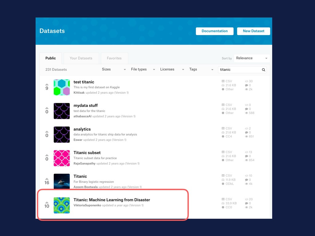
3. Kaggle is a place where you can find a lot of datasets, it already have installed most of tools you’ll need for a basic analysis, is a good place to see the people’s code and built a portfolio Why Kaggle?
4. Choosing a dataset https://www.kaggle.com/datasets
6. https://www.kaggle.com/vikichocolate/ titanic-machine-learning-from-disaster
9. Notebooks are a place where you can create code, show graphs, document your methodologies and findings… all in a single place
10. You can write code You can write text
11. And they work well together
12. Numbers on code cells indicate the order in which each cell ran
13. Notebooks always print the last line (event without the print statement)
14. Jupyter Shortcuts Ctrl + Enter = Run cell ESC + B = New cell below ESC + dd = Delete cell
15. Run the first cell
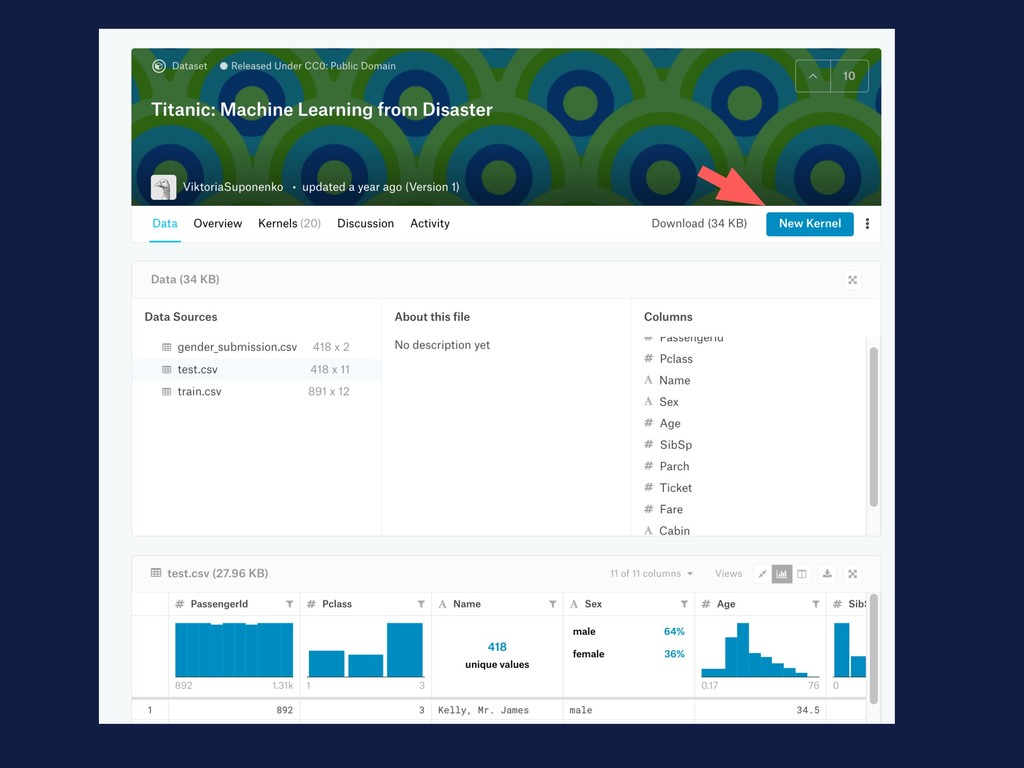
16. Reading a document If you check the first cell, it will tell you that the documents are ready for you in ../input/. So, we can read the files by with a Pandas function and with the path of the file df = pd.read_csv(‘../input/train.csv')
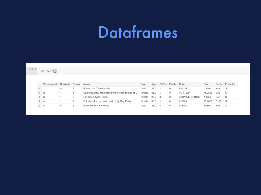
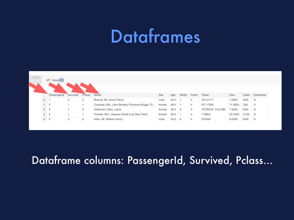
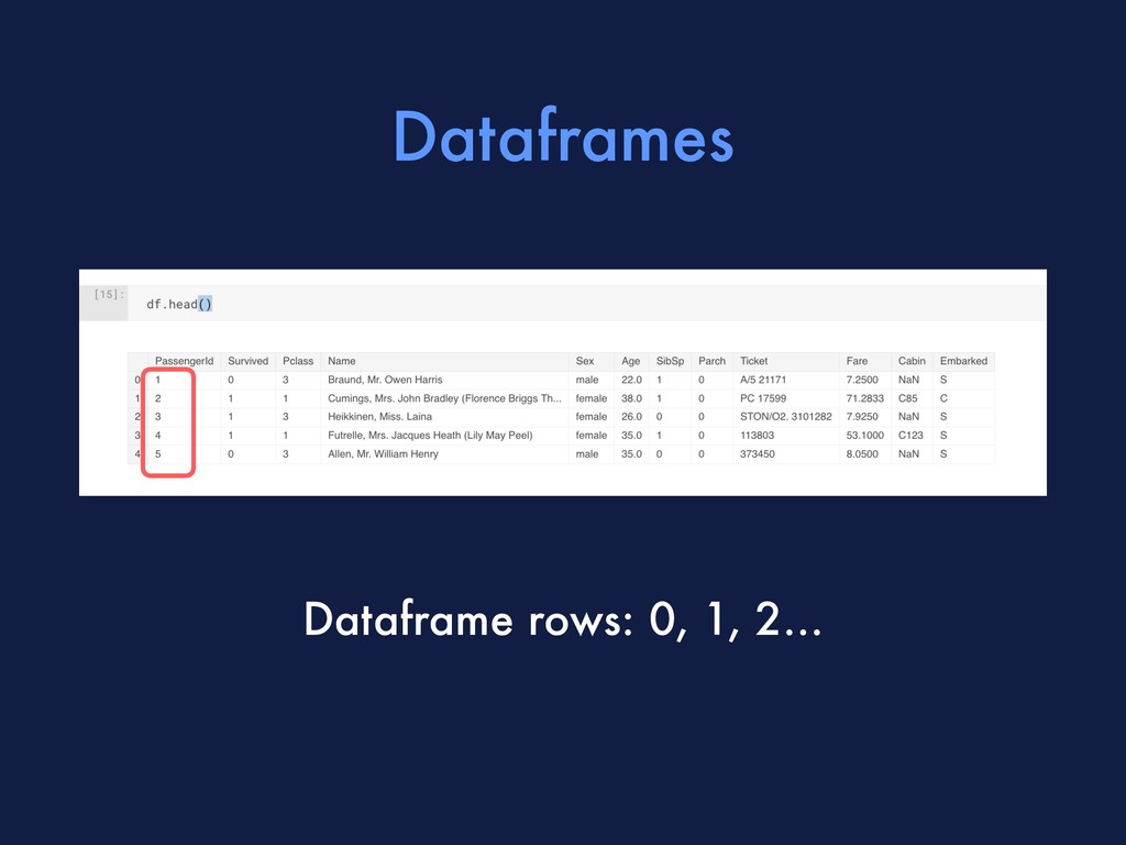
17. Dataframes Dataframes are similiar to what you find in Excel structures. You have rows indicated by numbers and columns with names. You can check the first 5 rows of a data frame to see the basic structure: df.head()
18. Dataframes
19. Dataframes Dataframe columns: PassengerId, Survived, Pclass…
20. Dataframes Dataframe rows: 0, 1, 2…
21. Dataframes You can check the structure of a dataframe, to get an idea of how many rows and columns it has: df.shape
22. Dataframes You can check the main statistical characteristics of the numerical columns of a data frame df.describe()
23. Dataframes df.describe()
24. Series You can select a single column of the data frame to work with. A column of a Dataframe is called Series and have some special properties df['Age']
25. Series You can also check the statistical characteristics of a Series df['Age'].describe()
26. Series You can filter a series to see which rows have adults. This will return a Series of True and False. df[‘Age'] > 10
27. Series And Series have functions that help you quickly plot some of it. We can, for instance, check the histogram of Ages. df[‘Age’].plot.hist()
28. Exercise Plot the histogram of Fares
29. Series And Series have functions that help you quickly plot some of it. We can, for instance, check the histogram of Ages. df[‘Age’].plot.hist()
30. Series We can count how many passengers were on each class df[‘Pclass’].value_counts()
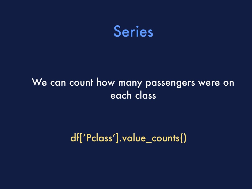
31. Series Since the result of a value_counts is also a Series, we can store this value in a variable and use it to plot a pie chart :) passengers_per_class = df[‘Pclass’].value_counts() passengers_per_class.plot.pie()
32. Exercise Plot a bar plot with the number of people that survived and didn’t survive (Column Survived)
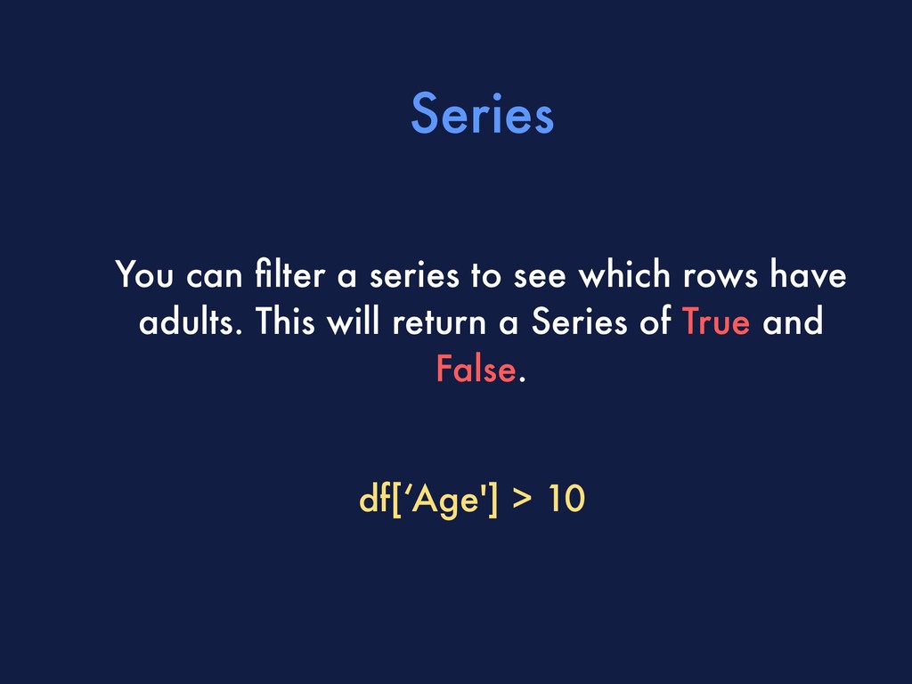
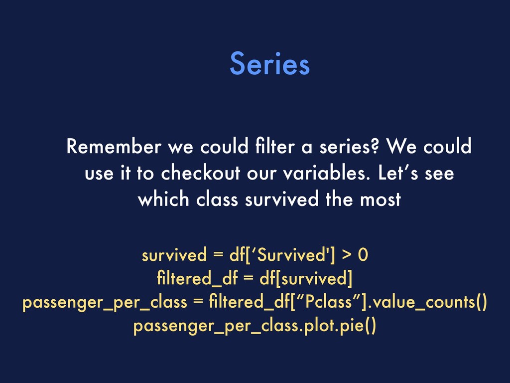
33. Series Remember we could filter a series? We could use it to checkout our variables. Let’s see which class survived the most survived = df[‘Survived'] > 0 filtered_df = df[survived] passenger_per_class = filtered_df[“Pclass”].value_counts() passenger_per_class.plot.pie()
34. Function Let’s build a function that “breaks" the age into classes:
35. Function Now if we pass an age to the function it returns a label:
36. Series We can create a new column (Ageclass) using the Column Age and this function :) df[“Ageclass”] = df[“Age”].apply(age_to_ageclass)
37. Exercise Now we have classes for age, we can check which sector survived the most, the same we did with Class :)
38. Dataframes We can group two columns to count df[“Ageclass”] = df[“Age”].apply(age_to_ageclass)