Lecture 10 - Metapopulation Models

Transcript

1. Metapopulation models
2. Metapopulations A metapopulation is a population of subpopulations linked by dispersal Introduction Abundance models Occupancy models Case study 2 / 24
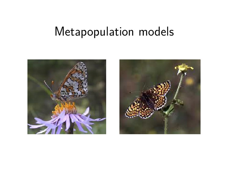
3. Metapopulations A metapopulation is a population of subpopulations linked by dispersal Properties • Subpopulations occur in discrete habitat patches • The landscape “matrix” is not suitable for reproduction Introduction Abundance models Occupancy models Case study 2 / 24
4. Motivation • Many populations are fragmented Introduction Abundance models Occupancy models Case study 3 / 24
5. Motivation • Many populations are fragmented • Metapopulation models can be used to forecast dynamics of fragmented populations Introduction Abundance models Occupancy models Case study 3 / 24
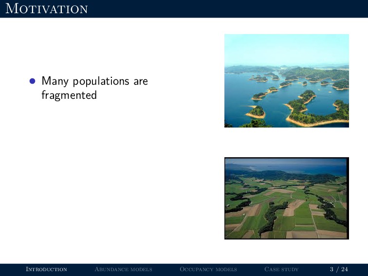
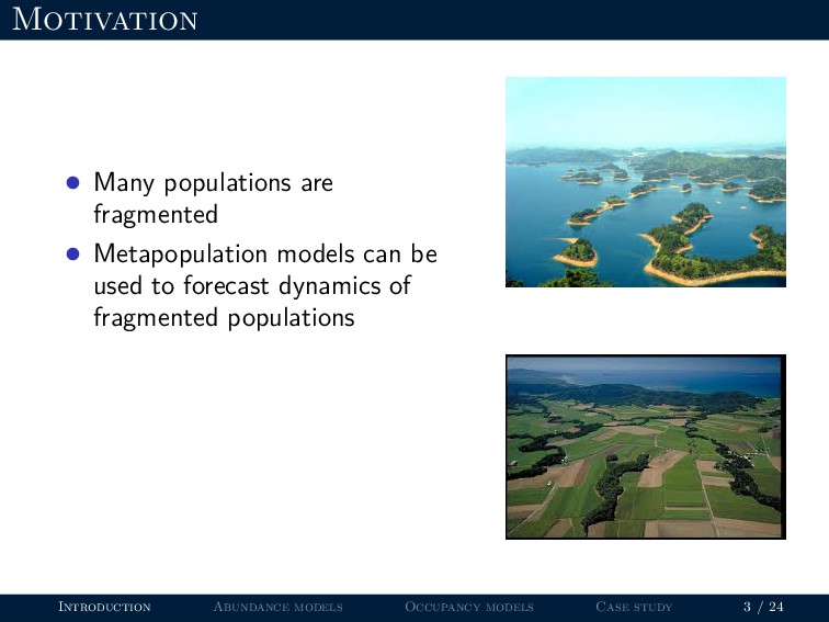
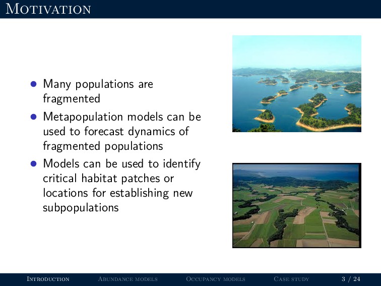
6. Motivation • Many populations are fragmented • Metapopulation models can be used to forecast dynamics of fragmented populations • Models can be used to identify critical habitat patches or locations for establishing new subpopulations Introduction Abundance models Occupancy models Case study 3 / 24
7. Origins Richard Levins First metapopulation models were parameterized in terms of the proportion of patches occupied Introduction Abundance models Occupancy models Case study 4 / 24
8. Origins Richard Levins First metapopulation models were parameterized in terms of the proportion of patches occupied Modern models are formulated in terms of patch-specific occupancy or abundance Introduction Abundance models Occupancy models Case study 4 / 24
9. Abundance formulation A simple case with only three subpopulations Nt = n1,t + n2,t + n3,t Introduction Abundance models Occupancy models Case study 5 / 24
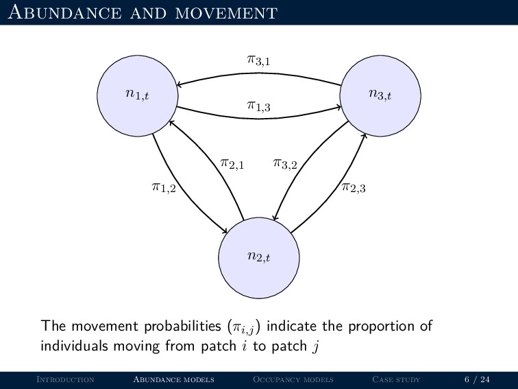
10. Abundance and movement n1,t n2,t n3,t π1,2 π2,1 π1,3 π3,1 π2,3 π3,2 The movement probabilities (πi,j) indicate the proportion of individuals moving from patch i to patch j Introduction Abundance models Occupancy models Case study 6 / 24
11. Abundance models Building the metapopulation model for the first subpopulation n1,t+1 = n1,t λ1 Three components (1) Geometric growth Introduction Abundance models Occupancy models Case study 7 / 24
12. Abundance models Building the metapopulation model for the first subpopulation n1,t+1 = n1,t λ1 (1 − π1,2 − π1,3 ) + Three components (1) Geometric growth (2) 1 minus emigration rates Introduction Abundance models Occupancy models Case study 7 / 24
13. Abundance models Building the metapopulation model for the first subpopulation n1,t+1 = n1,t λ1 (1 − π1,2 − π1,3 ) + n2,t λ2 (π2,1 ) + n3,t λ3 (π3,1 ) Three components (1) Geometric growth (2) 1 minus emigration rates (3) Immigration from subpopulations 2 and 3 Introduction Abundance models Occupancy models Case study 7 / 24
14. What influences movement? The movement probabilities (πi,j) represent the outcomes of both immigration and emigration. What influences these probabilities? Introduction Abundance models Occupancy models Case study 8 / 24
15. What influences movement? The movement probabilities (πi,j) represent the outcomes of both immigration and emigration. What influences these probabilities? Examples • Habitat quality in the patch of origin • Habitat quality in the landscape between origin and destination patches • Habitat quality in the destination patch • Distance between patches Introduction Abundance models Occupancy models Case study 8 / 24
16. Sources, sinks, and traps Source A patch with λ > 1. Sources tend to be net exporters of individuals. Introduction Abundance models Occupancy models Case study 9 / 24
17. Sources, sinks, and traps Source A patch with λ > 1. Sources tend to be net exporters of individuals. Sink A patch with λ < 1. Sinks would go extinct in the absence of immigration. Introduction Abundance models Occupancy models Case study 9 / 24
18. Sources, sinks, and traps Source A patch with λ > 1. Sources tend to be net exporters of individuals. Sink A patch with λ < 1. Sinks would go extinct in the absence of immigration. Ecological trap A sink that animals incorrectly perceive as a high quality source. Introduction Abundance models Occupancy models Case study 9 / 24
19. Density and habitat quality Can we identify sources, sinks, and traps by estimating patch-specific density (at one point in time)? Introduction Abundance models Occupancy models Case study 10 / 24
20. Density and habitat quality Can we identify sources, sinks, and traps by estimating patch-specific density (at one point in time)? Introduction Abundance models Occupancy models Case study 10 / 24
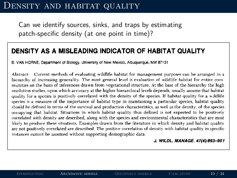
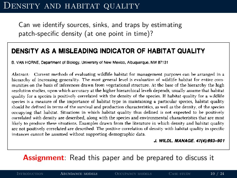
21. Density and habitat quality Can we identify sources, sinks, and traps by estimating patch-specific density (at one point in time)? Assignment: Read this paper and be prepared to discuss it Introduction Abundance models Occupancy models Case study 10 / 24
22. Occupancy models
23. Occupancy models Emphasis on stochastic patch-level dynamics • What is the probability that a patch will be occupied? Introduction Abundance models Occupancy models Case study 12 / 24
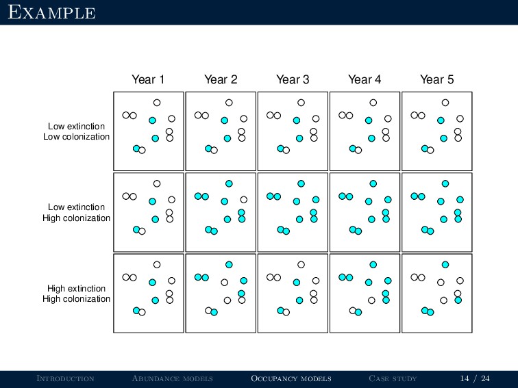
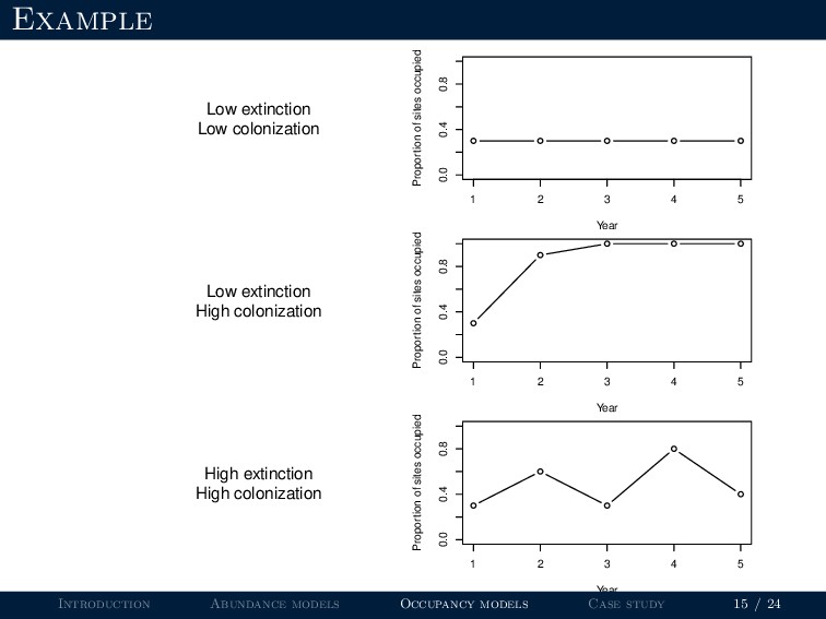
24. Occupancy models Emphasis on stochastic patch-level dynamics • What is the probability that a patch will be occupied? • What is the probability that an empty patch will be colonized? Introduction Abundance models Occupancy models Case study 12 / 24
25. Occupancy models Emphasis on stochastic patch-level dynamics • What is the probability that a patch will be occupied? • What is the probability that an empty patch will be colonized? • What is the probability that a subpopulation will go locally extinct? Introduction Abundance models Occupancy models Case study 12 / 24
26. Occupancy models Emphasis on stochastic patch-level dynamics • What is the probability that a patch will be occupied? • What is the probability that an empty patch will be colonized? • What is the probability that a subpopulation will go locally extinct? • What is the probability that the entire metapopulation will go extinct? Introduction Abundance models Occupancy models Case study 12 / 24
27. Definitions Occurrence (Oi,t) Indicates if patch i occupied at time t Introduction Abundance models Occupancy models Case study 13 / 24
28. Definitions Occurrence (Oi,t) Indicates if patch i occupied at time t Occurrence probability (psi=ψi,t) Probability that site i is occupied at time t Introduction Abundance models Occupancy models Case study 13 / 24
29. Definitions Occurrence (Oi,t) Indicates if patch i occupied at time t Occurrence probability (psi=ψi,t) Probability that site i is occupied at time t Colonization probability (gamma=γ) The probability that an unoccupied patch at time t becomes occupied at time t + 1 Introduction Abundance models Occupancy models Case study 13 / 24
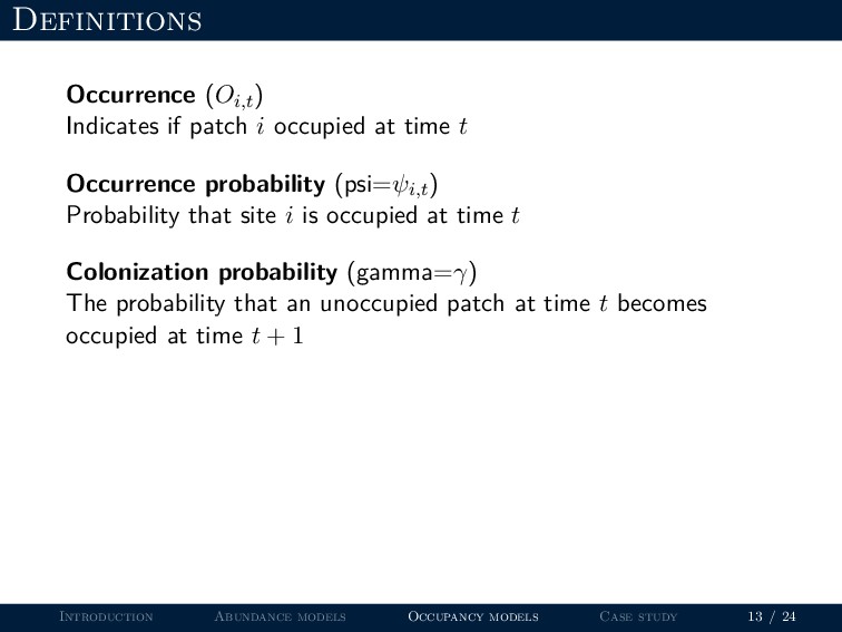
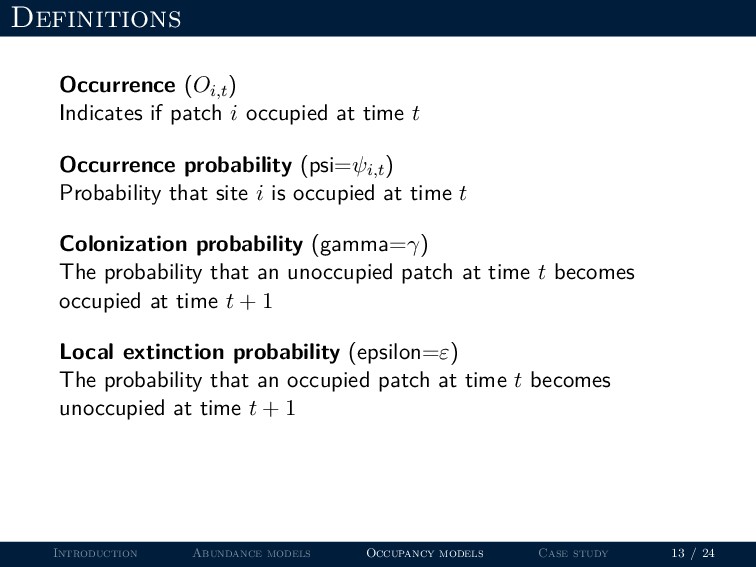
30. Definitions Occurrence (Oi,t) Indicates if patch i occupied at time t Occurrence probability (psi=ψi,t) Probability that site i is occupied at time t Colonization probability (gamma=γ) The probability that an unoccupied patch at time t becomes occupied at time t + 1 Local extinction probability (epsilon=ε) The probability that an occupied patch at time t becomes unoccupied at time t + 1 Introduction Abundance models Occupancy models Case study 13 / 24
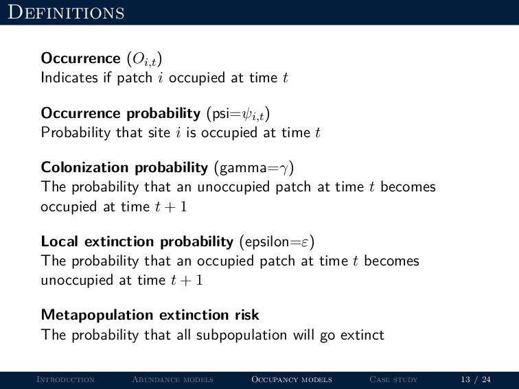
31. Definitions Occurrence (Oi,t) Indicates if patch i occupied at time t Occurrence probability (psi=ψi,t) Probability that site i is occupied at time t Colonization probability (gamma=γ) The probability that an unoccupied patch at time t becomes occupied at time t + 1 Local extinction probability (epsilon=ε) The probability that an occupied patch at time t becomes unoccupied at time t + 1 Metapopulation extinction risk The probability that all subpopulation will go extinct Introduction Abundance models Occupancy models Case study 13 / 24
32. Example Year 1 Year 2 Year 3 Year 4 Year 5 Low extinction Low colonization qq q q q q q q q q qq q q q q q q q q qq q q q q q q q q qq q q q q q q q q qq q q q q q q q q Low extinction High colonization qq q q q q q q q q qq q q q q q q q q qq q q q q q q q q qq q q q q q q q q qq q q q q q q q q High extinction High colonization qq q q q q q q q q qq q q q q q q q q qq q q q q q q q q qq q q q q q q q q qq q q q q q q q q Introduction Abundance models Occupancy models Case study 14 / 24
33. Example Low extinction Low colonization q q q q q 1 2 3 4 5 0.0 0.4 0.8 Year Proportion of sites occupied Low extinction High colonization q q q q q 1 2 3 4 5 0.0 0.4 0.8 Year Proportion of sites occupied High extinction High colonization q q q q q 1 2 3 4 5 0.0 0.4 0.8 Year Proportion of sites occupied Introduction Abundance models Occupancy models Case study 15 / 24
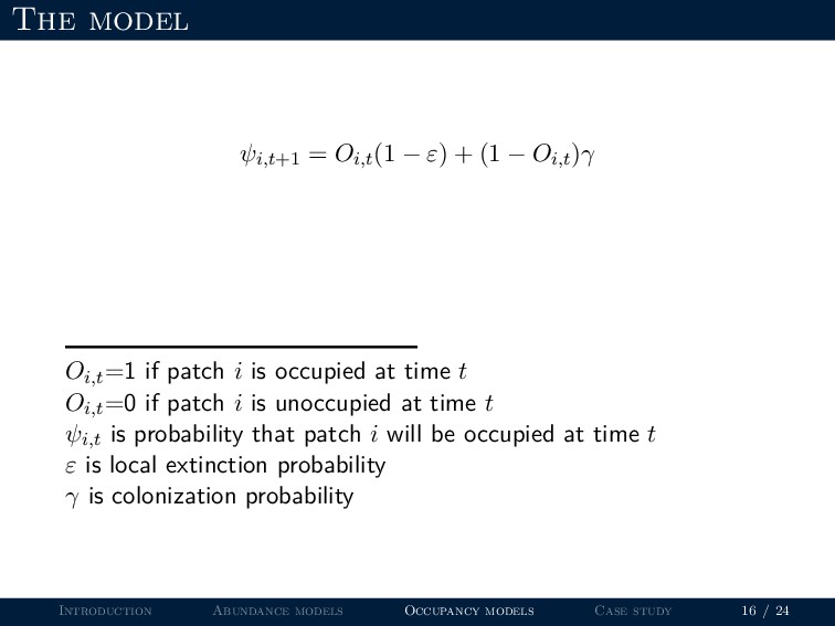
34. The model ψi,t+1 = Oi,t(1 − ε) + (1 − Oi,t)γ Oi,t=1 if patch i is occupied at time t Oi,t=0 if patch i is unoccupied at time t ψi,t is probability that patch i will be occupied at time t ε is local extinction probability γ is colonization probability Introduction Abundance models Occupancy models Case study 16 / 24
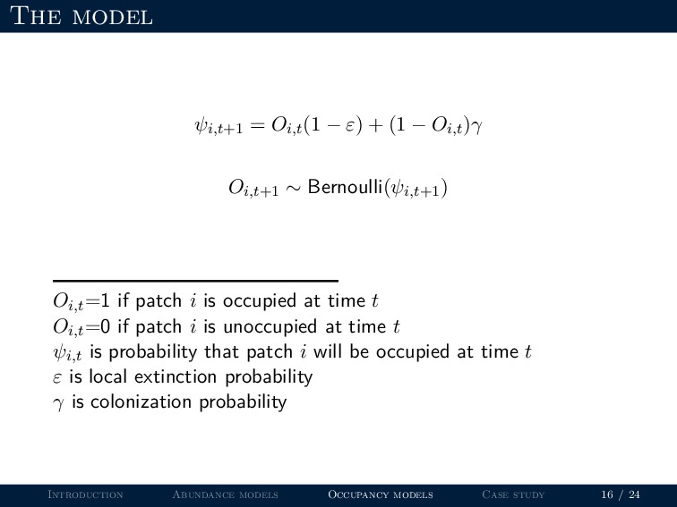
35. The model ψi,t+1 = Oi,t(1 − ε) + (1 − Oi,t)γ Oi,t+1 ∼ Bernoulli(ψi,t+1) Oi,t=1 if patch i is occupied at time t Oi,t=0 if patch i is unoccupied at time t ψi,t is probability that patch i will be occupied at time t ε is local extinction probability γ is colonization probability Introduction Abundance models Occupancy models Case study 16 / 24
36. Assumptions of basic non-spatial model • Abundance doesn’t matter • Patch quality is constant • Colonization and local extinction probabilities are constant • Landscape matrix doesn’t matter Introduction Abundance models Occupancy models Case study 17 / 24
37. Spatial models Introduction Abundance models Occupancy models Case study 18 / 24
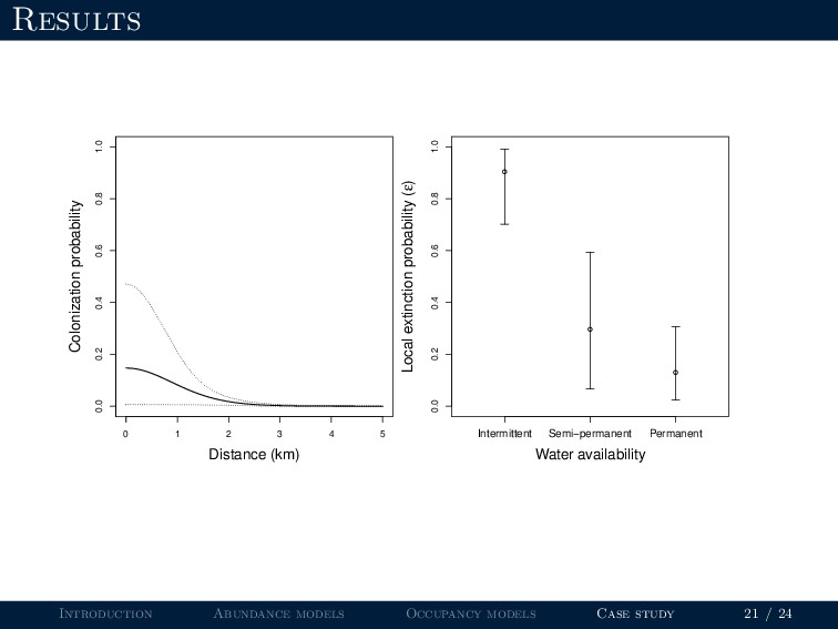
38. Spatial models All else equal. . . • An unoccupied site should have a higher chance of being colonized if it is close to an occupied site than if it is isolated Introduction Abundance models Occupancy models Case study 19 / 24
39. Spatial models All else equal. . . • An unoccupied site should have a higher chance of being colonized if it is close to an occupied site than if it is isolated • Similarly, isolated sites should have a higher extinction probability than connected sites (rescue effect) Introduction Abundance models Occupancy models Case study 19 / 24
40. Spatial models All else equal. . . • An unoccupied site should have a higher chance of being colonized if it is close to an occupied site than if it is isolated • Similarly, isolated sites should have a higher extinction probability than connected sites (rescue effect) • Connectivity is determined by Introduction Abundance models Occupancy models Case study 19 / 24
41. Spatial models All else equal. . . • An unoccupied site should have a higher chance of being colonized if it is close to an occupied site than if it is isolated • Similarly, isolated sites should have a higher extinction probability than connected sites (rescue effect) • Connectivity is determined by Dispersal ability Introduction Abundance models Occupancy models Case study 19 / 24
42. Spatial models All else equal. . . • An unoccupied site should have a higher chance of being colonized if it is close to an occupied site than if it is isolated • Similarly, isolated sites should have a higher extinction probability than connected sites (rescue effect) • Connectivity is determined by Dispersal ability Spatial configuration of sites Introduction Abundance models Occupancy models Case study 19 / 24
43. Spatial models All else equal. . . • An unoccupied site should have a higher chance of being colonized if it is close to an occupied site than if it is isolated • Similarly, isolated sites should have a higher extinction probability than connected sites (rescue effect) • Connectivity is determined by Dispersal ability Spatial configuration of sites Landscape resistance to movement Introduction Abundance models Occupancy models Case study 19 / 24
44. Spatial models All else equal. . . • An unoccupied site should have a higher chance of being colonized if it is close to an occupied site than if it is isolated • Similarly, isolated sites should have a higher extinction probability than connected sites (rescue effect) • Connectivity is determined by Dispersal ability Spatial configuration of sites Landscape resistance to movement • Modern models account for all of this Introduction Abundance models Occupancy models Case study 19 / 24
45. Case study Introduction Abundance models Occupancy models Case study 20 / 24
46. Results 0 1 2 3 4 5 0.0 0.2 0.4 0.6 0.8 1.0 Distance (km) Colonization probability q q q 0.0 0.2 0.4 0.6 0.8 1.0 Water availability Local extinction probability (ε) Intermittent Semi−permanent Permanent Introduction Abundance models Occupancy models Case study 21 / 24
47. Results Introduction Abundance models Occupancy models Case study 22 / 24
48. Results q q q q q q q q q q q q q q q q 2007 2010 2013 2016 2019 2022 0.0 0.2 0.4 0.6 0.8 1.0 Proportion of sites occupied q q q q q q q q q q q q q q q q 2007 2010 2013 2016 2019 2022 0.00 0.02 0.04 0.06 0.08 0.10 Metapopulation extinction probability Introduction Abundance models Occupancy models Case study 23 / 24
49. Summary Metapopulation models are widely used to describe the dynamics of fragmented populations Model can be formulated in terms of patch-level abundance and/or occupancy Modern models are stochastic and spatially explicit Introduction Abundance models Occupancy models Case study 24 / 24