Aude Sportisse

(CNRS, Computer Science Laboratory of Grenoble LIG)

Title — Safe semi-supervised learning when the labels are informative

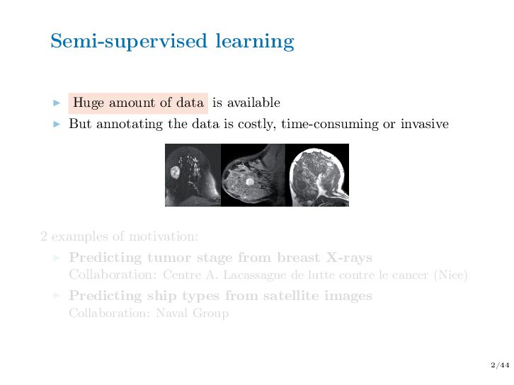
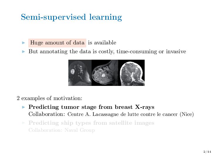
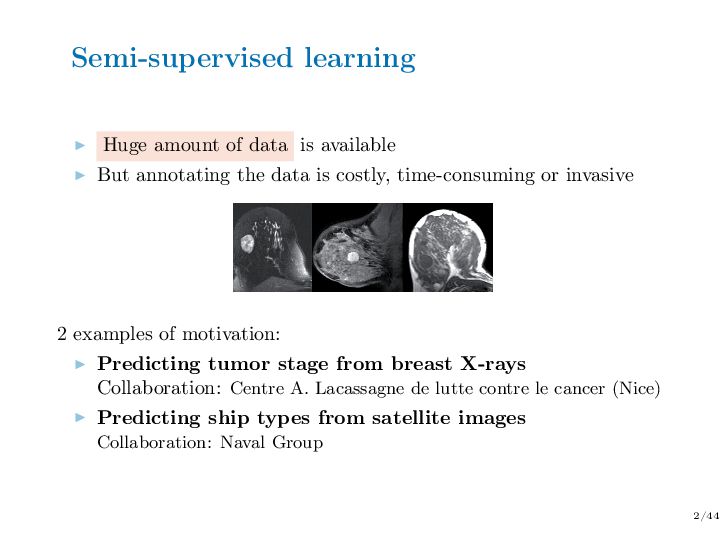
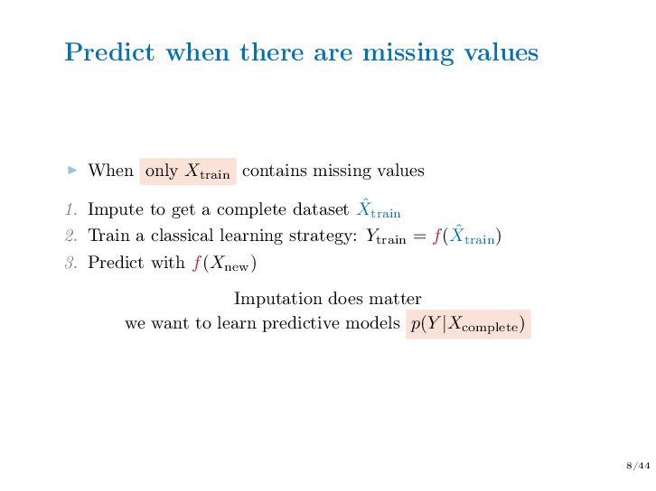
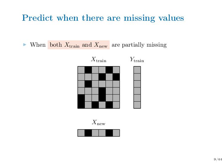
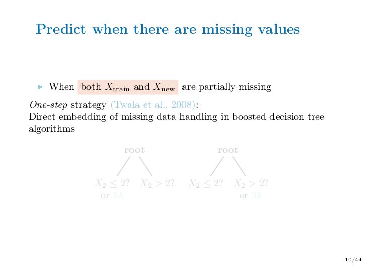
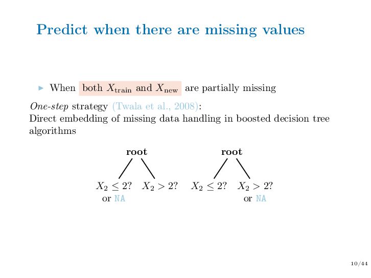
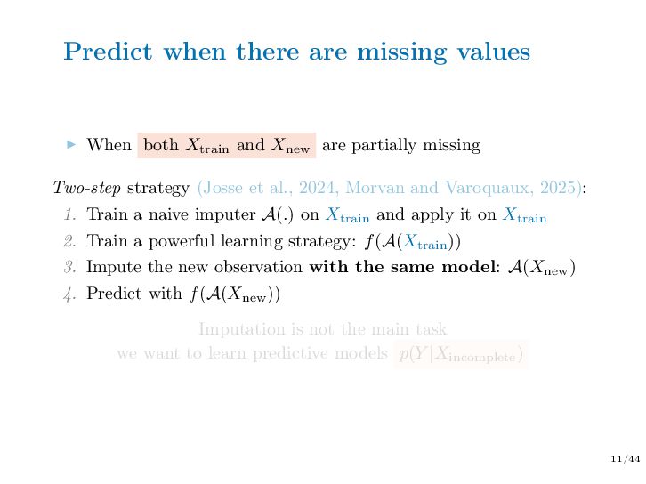
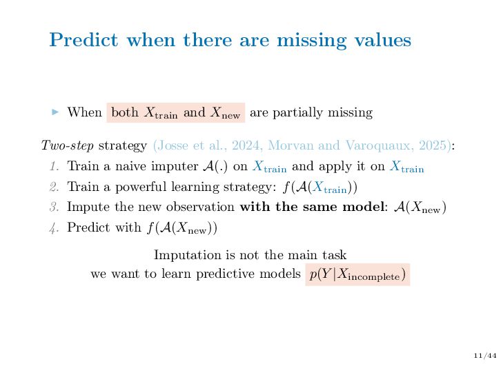
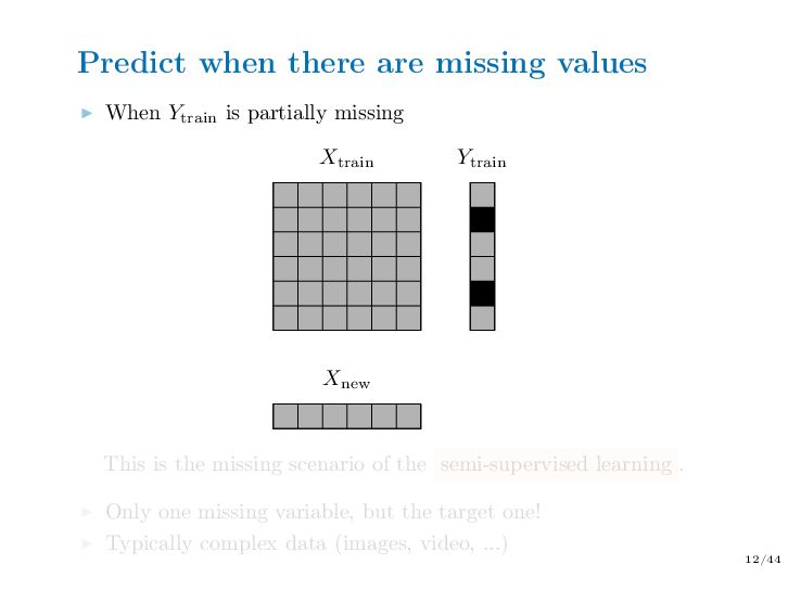
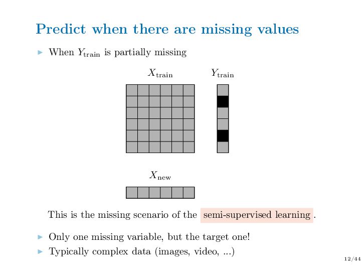
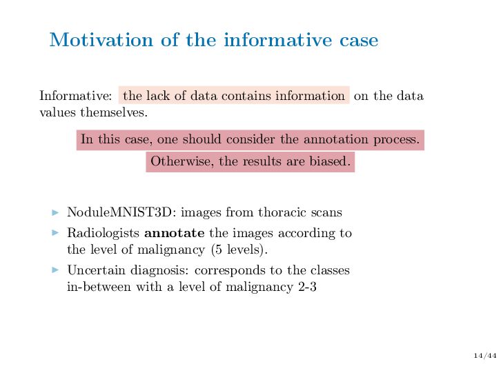
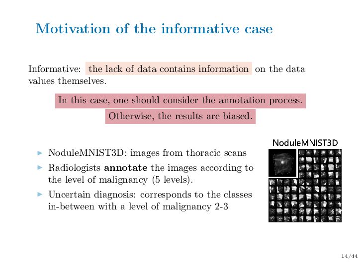
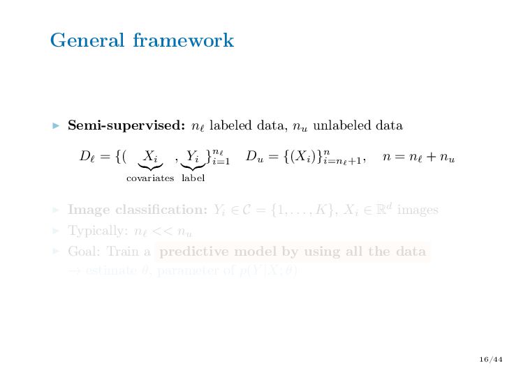
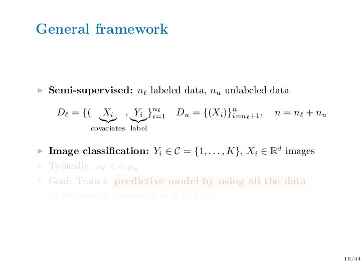
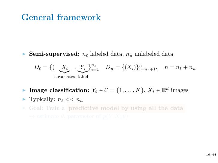
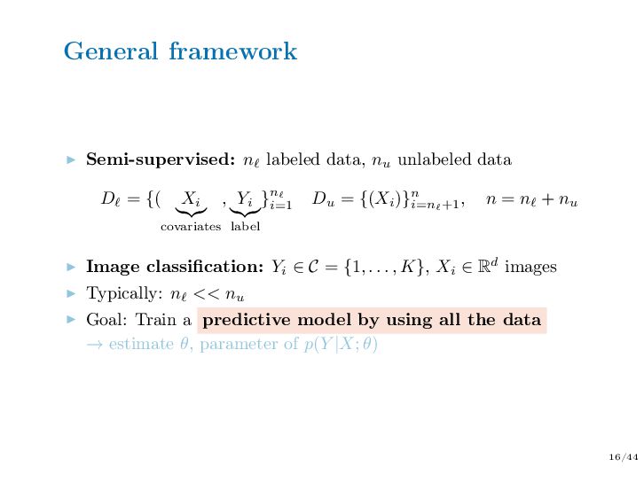
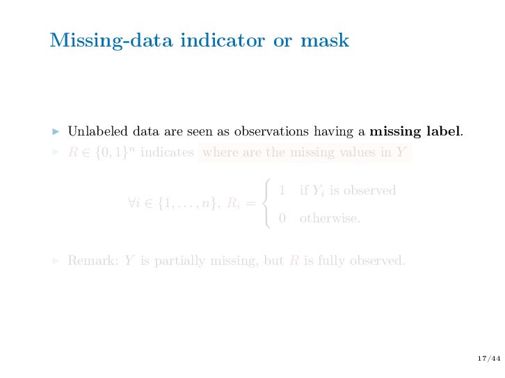
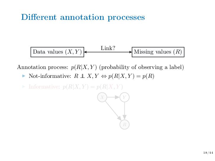
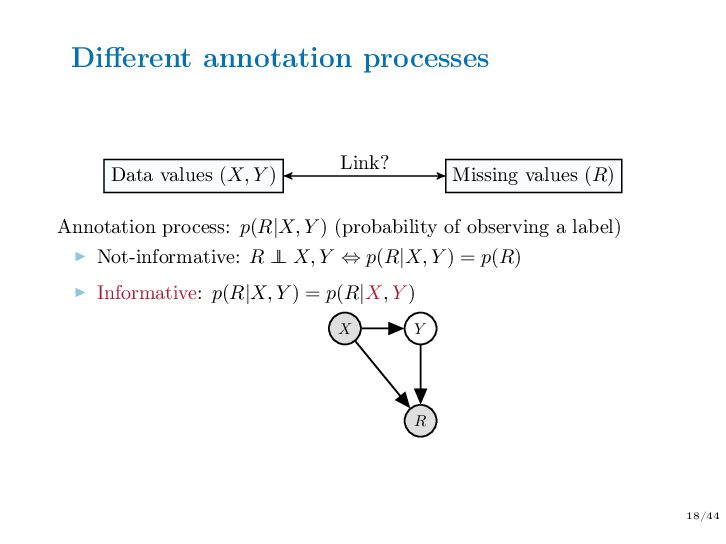
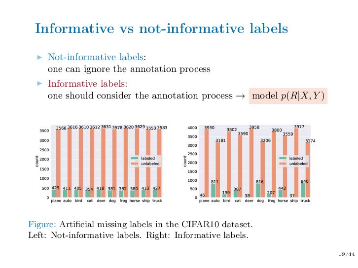
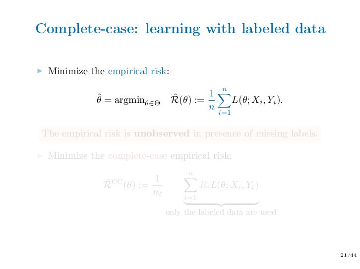
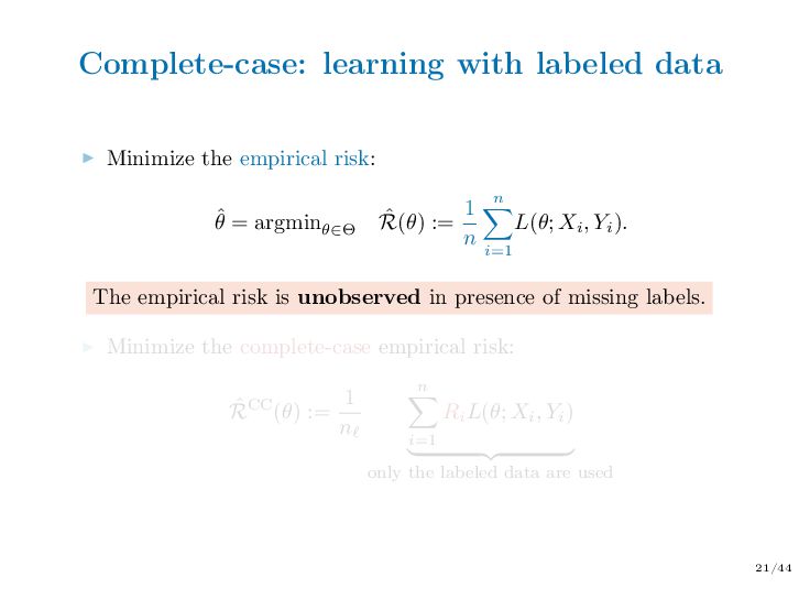
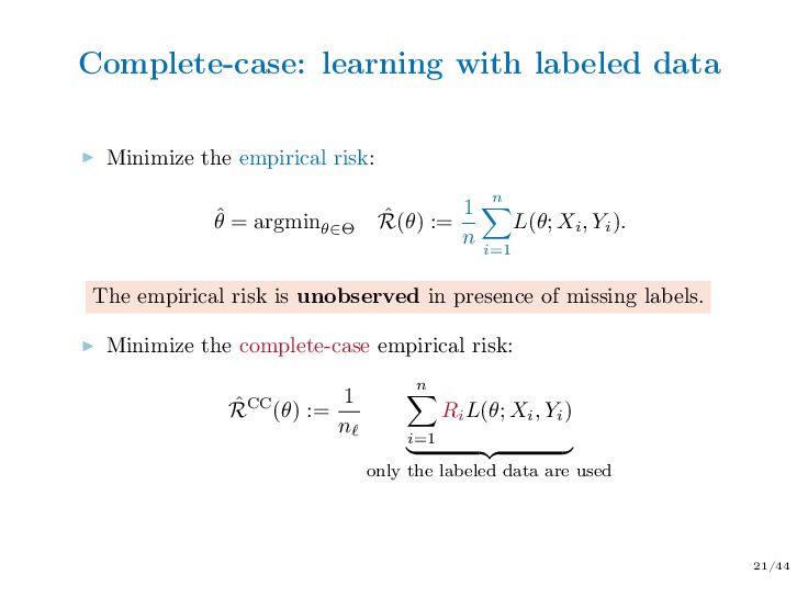
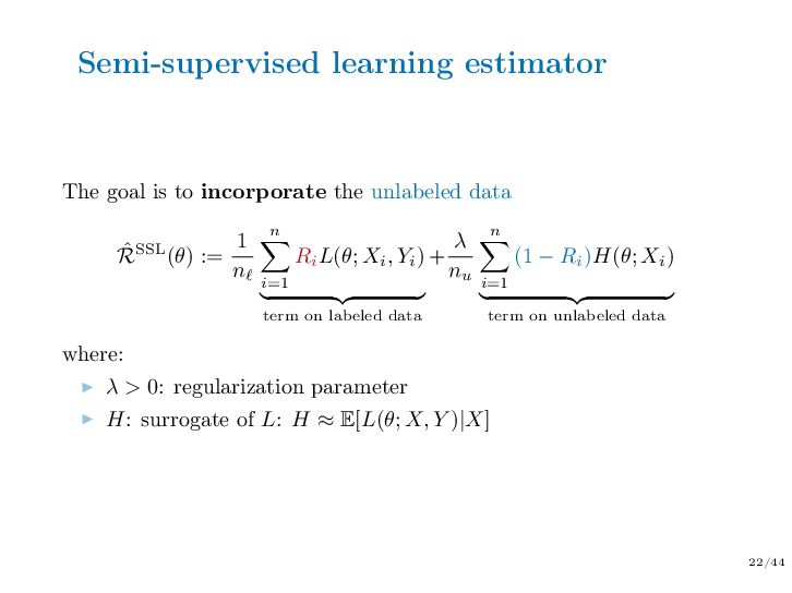
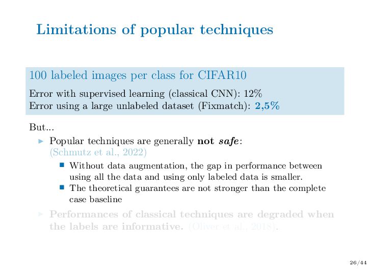
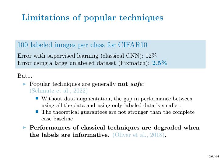
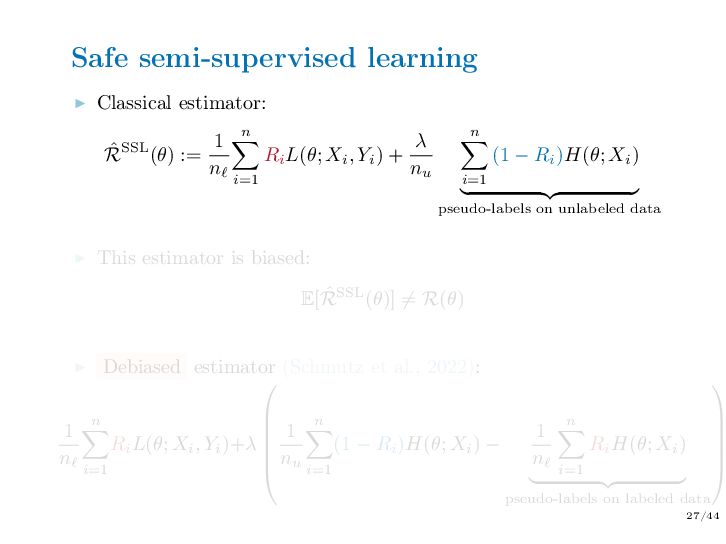
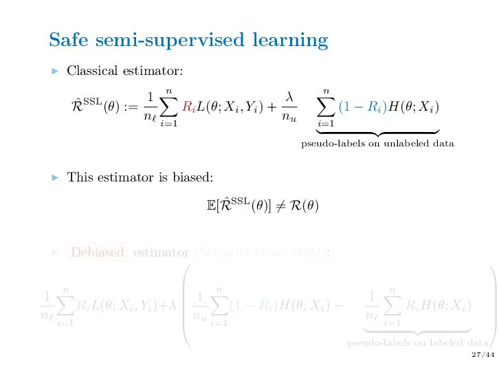
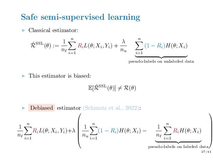
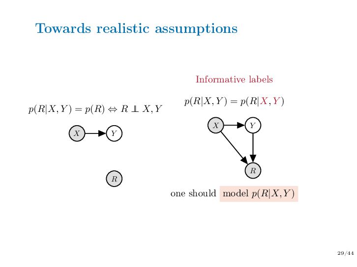
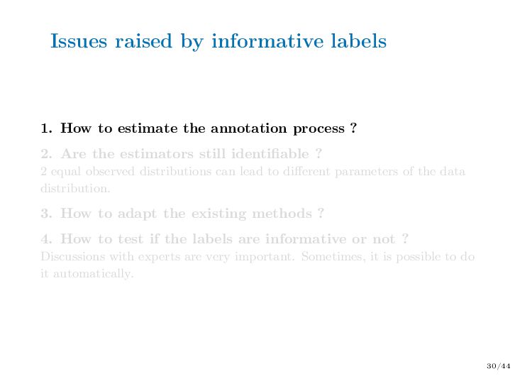
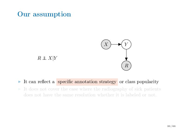
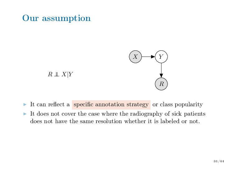
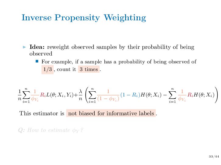
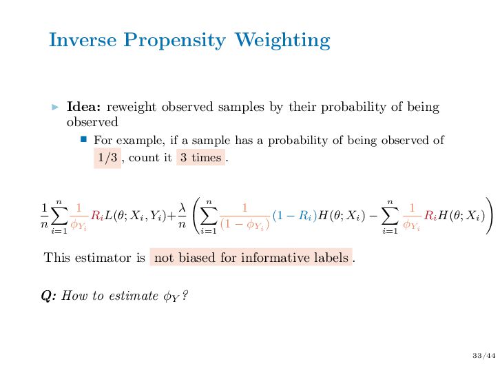
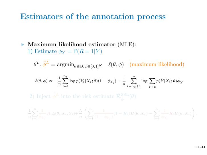
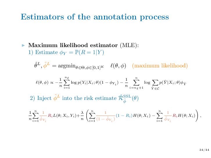
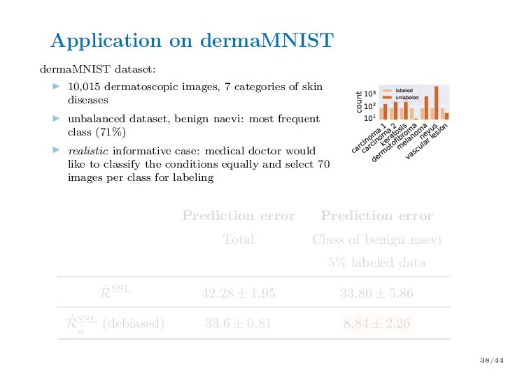
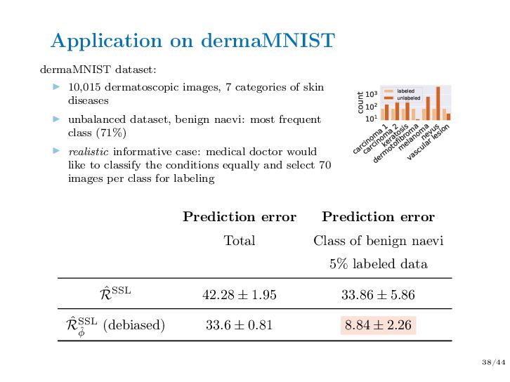
Abstract — In semi-supervised learning, we have access to features but the outcome variable is missing for a part of the data. In real life, although the amount of data available is often huge, labeling the data is costly and time-consuming. It is particularly true for image data sets: images are available in large quantities on image banks but they are most of the time unlabeled. It is therefore necessary to ask experts to label them. In this context, people are more inclined to label images of some classes which are easy to recognize. The unlabeled data are thus informative missing values, because the unavailability of the labels depends on their values themselves. Typically, the goal of semi-supervised learning is to learn predictive models using all the data (labeled and unlabeled ones). However, classical methods lead to biased estimates if the missing values are informative. We aim at designing new semi-supervised algorithms that handle informative missing labels.

Bio
Since October 2024, I am a CNRS researcher in the APTIKAL team of the Computer Science Laboratory of Grenoble LIG. From October 2023 to the end of Septembrer 2024, I was a junior fellow in Efelia Côte d’Azur. From October 2021 to the end of September 2023, I was a Postdoctoral researcher of the 3iA Côte d’Azur at Centre Inria d’Université Côte d’Azur in the Maasai team. I was working on deep semi-supervised learning, with Charles Bouveyron and Pierre-Alexandre Mattei. My PhD thesis (2018-2021) in Applied Mathematics was supervised by Claire Boyer and Julie Josse at Ecole Polytechnique (CMAP) and University Pierre and Marie Curie (LPSM).

Transcript

1. 1/44 Safe semi-supervised learning with biased labels Aude Sportisse <aude.sportisse@univ-grenoble-alpes.fr> CNRS researcher Laboratoire d’Informatique de Grenoble, APTIKAL Team
2. 2/44 Semi-supervised learning ▶ Huge amount of data is available ▶ But annotating the data is costly, time-consuming or invasive 2 examples of motivation: ▶ Predicting tumor stage from breast X-rays Collaboration: Centre A. Lacassagne de lutte contre le cancer (Nice) ▶ Predicting ship types from satellite images Collaboration: Naval Group
3. 2/44 Semi-supervised learning ▶ Huge amount of data is available ▶ But annotating the data is costly, time-consuming or invasive 2 examples of motivation: ▶ Predicting tumor stage from breast X-rays Collaboration: Centre A. Lacassagne de lutte contre le cancer (Nice) ▶ Predicting ship types from satellite images Collaboration: Naval Group
4. 2/44 Semi-supervised learning ▶ Huge amount of data is available ▶ But annotating the data is costly, time-consuming or invasive 2 examples of motivation: ▶ Predicting tumor stage from breast X-rays Collaboration: Centre A. Lacassagne de lutte contre le cancer (Nice) ▶ Predicting ship types from satellite images Collaboration: Naval Group
5. 3/44 Toy datasets Figure: CIFAR10 dataset Figure: MedMNIST: datasets for 2D and 3D Biomedical Image Classification
6. 4/44 Plan Why is semi-supervised learning a missing-data problem ? How to leverage unlabeled data? What is safe semi-supervised learning? How to handle biased labels? Conclusion
7. 5/44 Supervised learning task ▶ From a new observation Xnew , predict a variable Ynew ▶ Training set: (Xtrain , Ytrain ) Xtrain Ytrain Xnew
8. 6/44 Predict when there are missing values First high-level question on the missingness scenario: Q: Where are the missing values, in Xtrain , Xnew , or Ytrain ?
9. 7/44 Predict when there are missing values ▶ When only Xtrain contains missing values Xtrain Ytrain Xnew
10. 8/44 Predict when there are missing values ▶ When only Xtrain contains missing values 1. Impute to get a complete dataset ˆ Xtrain 2. Train a classical learning strategy: Ytrain = f( ˆ Xtrain ) 3. Predict with f(Xnew ) Imputation does matter we want to learn predictive models p(Y |Xcomplete )
11. 8/44 Predict when there are missing values ▶ When only Xtrain contains missing values 1. Impute to get a complete dataset ˆ Xtrain 2. Train a classical learning strategy: Ytrain = f( ˆ Xtrain ) 3. Predict with f(Xnew ) Imputation does matter we want to learn predictive models p(Y |Xcomplete )
12. 8/44 Predict when there are missing values ▶ When only Xtrain contains missing values 1. Impute to get a complete dataset ˆ Xtrain 2. Train a classical learning strategy: Ytrain = f( ˆ Xtrain ) 3. Predict with f(Xnew ) Imputation does matter we want to learn predictive models p(Y |Xcomplete )
13. 8/44 Predict when there are missing values ▶ When only Xtrain contains missing values 1. Impute to get a complete dataset ˆ Xtrain 2. Train a classical learning strategy: Ytrain = f( ˆ Xtrain ) 3. Predict with f(Xnew ) Imputation does matter we want to learn predictive models p(Y |Xcomplete )
14. 8/44 Predict when there are missing values ▶ When only Xtrain contains missing values 1. Impute to get a complete dataset ˆ Xtrain 2. Train a classical learning strategy: Ytrain = f( ˆ Xtrain ) 3. Predict with f(Xnew ) Imputation does matter we want to learn predictive models p(Y |Xcomplete )
15. 9/44 Predict when there are missing values ▶ When both Xtrain and Xnew are partially missing Xtrain Ytrain Xnew
16. 10/44 Predict when there are missing values ▶ When both Xtrain and Xnew are partially missing One-step strategy (Twala et al., 2008): Direct embedding of missing data handling in boosted decision tree algorithms root X2 ≤ 2? X2 > 2? or NA root X2 ≤ 2? X2 > 2? or NA
17. 10/44 Predict when there are missing values ▶ When both Xtrain and Xnew are partially missing One-step strategy (Twala et al., 2008): Direct embedding of missing data handling in boosted decision tree algorithms root X2 ≤ 2? X2 > 2? or NA root X2 ≤ 2? X2 > 2? or NA
18. 11/44 Predict when there are missing values ▶ When both Xtrain and Xnew are partially missing Two-step strategy (Josse et al., 2024, Morvan and Varoquaux, 2025): 1. Train a naive imputer A(.) on Xtrain and apply it on Xtrain 2. Train a powerful learning strategy: f(A(Xtrain )) 3. Impute the new observation with the same model: A(Xnew ) 4. Predict with f(A(Xnew )) Imputation is not the main task we want to learn predictive models p(Y |Xincomplete )
19. 11/44 Predict when there are missing values ▶ When both Xtrain and Xnew are partially missing Two-step strategy (Josse et al., 2024, Morvan and Varoquaux, 2025): 1. Train a naive imputer A(.) on Xtrain and apply it on Xtrain 2. Train a powerful learning strategy: f(A(Xtrain )) 3. Impute the new observation with the same model: A(Xnew ) 4. Predict with f(A(Xnew )) Imputation is not the main task we want to learn predictive models p(Y |Xincomplete )
20. 11/44 Predict when there are missing values ▶ When both Xtrain and Xnew are partially missing Two-step strategy (Josse et al., 2024, Morvan and Varoquaux, 2025): 1. Train a naive imputer A(.) on Xtrain and apply it on Xtrain 2. Train a powerful learning strategy: f(A(Xtrain )) 3. Impute the new observation with the same model: A(Xnew ) 4. Predict with f(A(Xnew )) Imputation is not the main task we want to learn predictive models p(Y |Xincomplete )
21. 11/44 Predict when there are missing values ▶ When both Xtrain and Xnew are partially missing Two-step strategy (Josse et al., 2024, Morvan and Varoquaux, 2025): 1. Train a naive imputer A(.) on Xtrain and apply it on Xtrain 2. Train a powerful learning strategy: f(A(Xtrain )) 3. Impute the new observation with the same model: A(Xnew ) 4. Predict with f(A(Xnew )) Imputation is not the main task we want to learn predictive models p(Y |Xincomplete )
22. 11/44 Predict when there are missing values ▶ When both Xtrain and Xnew are partially missing Two-step strategy (Josse et al., 2024, Morvan and Varoquaux, 2025): 1. Train a naive imputer A(.) on Xtrain and apply it on Xtrain 2. Train a powerful learning strategy: f(A(Xtrain )) 3. Impute the new observation with the same model: A(Xnew ) 4. Predict with f(A(Xnew )) Imputation is not the main task we want to learn predictive models p(Y |Xincomplete )
23. 11/44 Predict when there are missing values ▶ When both Xtrain and Xnew are partially missing Two-step strategy (Josse et al., 2024, Morvan and Varoquaux, 2025): 1. Train a naive imputer A(.) on Xtrain and apply it on Xtrain 2. Train a powerful learning strategy: f(A(Xtrain )) 3. Impute the new observation with the same model: A(Xnew ) 4. Predict with f(A(Xnew )) Imputation is not the main task we want to learn predictive models p(Y |Xincomplete )
24. 12/44 Predict when there are missing values ▶ When Ytrain is partially missing Xtrain Ytrain Xnew This is the missing scenario of the semi-supervised learning . ▶ Only one missing variable, but the target one! ▶ Typically complex data (images, video, ...)
25. 12/44 Predict when there are missing values ▶ When Ytrain is partially missing Xtrain Ytrain Xnew This is the missing scenario of the semi-supervised learning . ▶ Only one missing variable, but the target one! ▶ Typically complex data (images, video, ...)
26. 13/44 Predict when there are missing values Two specific questions on the missingness scenario: Q: Where exactly are the missing values? Q: Why are there missing values?
27. 13/44 Predict when there are missing values Two specific questions on the missingness scenario: Q: Where are exactly the missing values? → Easy task: introduce a binary variable that indicates where the missing data are. Q: Why are there missing values? → Difficult but important to know: understand the causal links between the missingness and the data values. → The missingness can be biased : the labeled data do not represent well the whole data. Biased missingness is also informative .
28. 14/44 Motivation of the informative case Informative: the lack of data contains information on the data values themselves. In this case, one should consider the annotation process. Otherwise, the results are biased. ▶ NoduleMNIST3D: images from thoracic scans ▶ Radiologists annotate the images according to the level of malignancy (5 levels). ▶ Uncertain diagnosis: corresponds to the classes in-between with a level of malignancy 2-3
29. 14/44 Motivation of the informative case Informative: the lack of data contains information on the data values themselves. In this case, one should consider the annotation process. Otherwise, the results are biased. ▶ NoduleMNIST3D: images from thoracic scans ▶ Radiologists annotate the images according to the level of malignancy (5 levels). ▶ Uncertain diagnosis: corresponds to the classes in-between with a level of malignancy 2-3
30. 14/44 Motivation of the informative case Informative: the lack of data contains information on the data values themselves. In this case, one should consider the annotation process. Otherwise, the results are biased. ▶ NoduleMNIST3D: images from thoracic scans ▶ Radiologists annotate the images according to the level of malignancy (5 levels). ▶ Uncertain diagnosis: corresponds to the classes in-between with a level of malignancy 2-3
31. 14/44 Motivation of the informative case Informative: the lack of data contains information on the data values themselves. In this case, one should consider the annotation process. Otherwise, the results are biased. ▶ NoduleMNIST3D: images from thoracic scans ▶ Radiologists annotate the images according to the level of malignancy (5 levels). ▶ Uncertain diagnosis: corresponds to the classes in-between with a level of malignancy 2-3
32. 15/44 Plan Why is semi-supervised learning a missing-data problem ? How to leverage unlabeled data? What is safe semi-supervised learning? How to handle biased labels? Conclusion
33. 16/44 General framework ▶ Semi-supervised: nℓ labeled data, nu unlabeled data Dℓ = {( Xi covariates , Yi label }nℓ i=1 Du = {(Xi )}n i=nℓ+1 , n = nℓ + nu ▶ Image classification: Yi ∈ C = {1, . . . , K}, Xi ∈ Rd images ▶ Typically: nℓ << nu ▶ Goal: Train a predictive model by using all the data → estimate θ, parameter of p(Y |X; θ)
34. 16/44 General framework ▶ Semi-supervised: nℓ labeled data, nu unlabeled data Dℓ = {( Xi covariates , Yi label }nℓ i=1 Du = {(Xi )}n i=nℓ+1 , n = nℓ + nu ▶ Image classification: Yi ∈ C = {1, . . . , K}, Xi ∈ Rd images ▶ Typically: nℓ << nu ▶ Goal: Train a predictive model by using all the data → estimate θ, parameter of p(Y |X; θ)
35. 16/44 General framework ▶ Semi-supervised: nℓ labeled data, nu unlabeled data Dℓ = {( Xi covariates , Yi label }nℓ i=1 Du = {(Xi )}n i=nℓ+1 , n = nℓ + nu ▶ Image classification: Yi ∈ C = {1, . . . , K}, Xi ∈ Rd images ▶ Typically: nℓ << nu ▶ Goal: Train a predictive model by using all the data → estimate θ, parameter of p(Y |X; θ)
36. 16/44 General framework ▶ Semi-supervised: nℓ labeled data, nu unlabeled data Dℓ = {( Xi covariates , Yi label }nℓ i=1 Du = {(Xi )}n i=nℓ+1 , n = nℓ + nu ▶ Image classification: Yi ∈ C = {1, . . . , K}, Xi ∈ Rd images ▶ Typically: nℓ << nu ▶ Goal: Train a predictive model by using all the data → estimate θ, parameter of p(Y |X; θ)
37. 17/44 Missing-data indicator or mask ▶ Unlabeled data are seen as observations having a missing label. ▶ R ∈ {0, 1}n indicates where are the missing values in Y ∀i ∈ {1, . . . , n}, Ri =    1 if Yi is observed 0 otherwise. ▶ Remark: Y is partially missing, but R is fully observed.
38. 17/44 Missing-data indicator or mask ▶ Unlabeled data are seen as observations having a missing label. ▶ R ∈ {0, 1}n indicates where are the missing values in Y ∀i ∈ {1, . . . , n}, Ri =    1 if Yi is observed 0 otherwise. ▶ Remark: Y is partially missing, but R is fully observed.
39. 17/44 Missing-data indicator or mask ▶ Unlabeled data are seen as observations having a missing label. ▶ R ∈ {0, 1}n indicates where are the missing values in Y ∀i ∈ {1, . . . , n}, Ri =    1 if Yi is observed 0 otherwise. ▶ Remark: Y is partially missing, but R is fully observed.
40. 18/44 Different annotation processes Data values (X, Y ) Missing values (R) Link? Annotation process: p(R|X, Y ) (probability of observing a label) ▶ Not-informative: R ⊥ ⊥ X, Y ⇔ p(R|X, Y ) = p(R) ▶ Informative: p(R|X, Y ) = p(R|X, Y ) X Y R
41. 18/44 Different annotation processes Data values (X, Y ) Missing values (R) Link? Annotation process: p(R|X, Y ) (probability of observing a label) ▶ Not-informative: R ⊥ ⊥ X, Y ⇔ p(R|X, Y ) = p(R) ▶ Informative: p(R|X, Y ) = p(R|X, Y ) X Y R
42. 18/44 Different annotation processes Data values (X, Y ) Missing values (R) Link? Annotation process: p(R|X, Y ) (probability of observing a label) ▶ Not-informative: R ⊥ ⊥ X, Y ⇔ p(R|X, Y ) = p(R) ▶ Informative: p(R|X, Y ) = p(R|X, Y ) X Y R
43. 18/44 Different annotation processes Data values (X, Y ) Missing values (R) Link? Annotation process: p(R|X, Y ) (probability of observing a label) ▶ Not-informative: R ⊥ ⊥ X, Y ⇔ p(R|X, Y ) = p(R) ▶ Informative: p(R|X, Y ) = p(R|X, Y ) X Y R
44. 19/44 Informative vs not-informative labels ▶ Not-informative labels: one can ignore the annotation process ▶ Informative labels: one should consider the annotation process → model p(R|X, Y )
45. 19/44 Informative vs not-informative labels ▶ Not-informative labels: one can ignore the annotation process ▶ Informative labels: one should consider the annotation process → model p(R|X, Y )
46. 19/44 Informative vs not-informative labels ▶ Not-informative labels: one can ignore the annotation process ▶ Informative labels: one should consider the annotation process → model p(R|X, Y ) plane auto bird cat deer dog frog horse ship truck 0 500 1000 1500 2000 2500 3000 3500 count 429 411 405 354 418 381 382 380 413 427 3568 3616 3610 3612 3631 3578 3620 3629 3553 3583 labeled unlabeled plane auto bird cat deer dog frog horse ship truck 0 500 1000 1500 2000 2500 3000 3500 4000 count 46 811 199 387 38 816 207 442 37 840 3930 3181 3802 3590 3958 3206 3800 3559 3977 3174 labeled unlabeled Figure: Artificial missing labels in the CIFAR10 dataset. Left: Not-informative labels. Right: Informative labels.
47. 20/44 Objective in semi-supervised learning ▶ Focus on the not-informative case ▶ Objective: train a predictive model p(Y |X; θ) ▶ Two modeling components: ▪ Negative log-likelihood: L(θ, X, Y ) = − log p(Y |X; θ). ▪ p(Y |X; θ) is typically a convolutional neural network . ▶ The oracle estimate is the minimizer of the theoretical risk: θ⋆ = argminθ∈Θ R(θ) := E(X,Y )∼p(X,Y ) [L(θ; X, Y )]. The theoretical risk is always intractable.
48. 20/44 Objective in semi-supervised learning ▶ Focus on the not-informative case ▶ Objective: train a predictive model p(Y |X; θ) ▶ Two modeling components: ▪ Negative log-likelihood: L(θ, X, Y ) = − log p(Y |X; θ). ▪ p(Y |X; θ) is typically a convolutional neural network . ▶ The oracle estimate is the minimizer of the theoretical risk: θ⋆ = argminθ∈Θ R(θ) := E(X,Y )∼p(X,Y ) [L(θ; X, Y )]. The theoretical risk is always intractable.
49. 20/44 Objective in semi-supervised learning ▶ Focus on the not-informative case ▶ Objective: train a predictive model p(Y |X; θ) ▶ Two modeling components: ▪ Negative log-likelihood: L(θ, X, Y ) = − log p(Y |X; θ). ▪ p(Y |X; θ) is typically a convolutional neural network . ▶ The oracle estimate is the minimizer of the theoretical risk: θ⋆ = argminθ∈Θ R(θ) := E(X,Y )∼p(X,Y ) [L(θ; X, Y )]. The theoretical risk is always intractable.
50. 21/44 Complete-case: learning with labeled data ▶ Minimize the empirical risk: ˆ θ = argminθ∈Θ ˆ R(θ) := 1 n n i=1 L(θ; Xi , Yi ). The empirical risk is unobserved in presence of missing labels. ▶ Minimize the complete-case empirical risk: ˆ RCC(θ) := 1 nℓ n i=1 Ri L(θ; Xi , Yi ) only the labeled data are used
51. 21/44 Complete-case: learning with labeled data ▶ Minimize the empirical risk: ˆ θ = argminθ∈Θ ˆ R(θ) := 1 n n i=1 L(θ; Xi , Yi ). The empirical risk is unobserved in presence of missing labels. ▶ Minimize the complete-case empirical risk: ˆ RCC(θ) := 1 nℓ n i=1 Ri L(θ; Xi , Yi ) only the labeled data are used
52. 21/44 Complete-case: learning with labeled data ▶ Minimize the empirical risk: ˆ θ = argminθ∈Θ ˆ R(θ) := 1 n n i=1 L(θ; Xi , Yi ). The empirical risk is unobserved in presence of missing labels. ▶ Minimize the complete-case empirical risk: ˆ RCC(θ) := 1 nℓ n i=1 Ri L(θ; Xi , Yi ) only the labeled data are used
53. 22/44 Semi-supervised learning estimator The goal is to incorporate the unlabeled data ˆ RSSL(θ) := 1 nℓ n i=1 Ri L(θ; Xi , Yi ) term on labeled data + λ nu n i=1 (1 − Ri )H(θ; Xi ) term on unlabeled data where: ▶ λ > 0: regularization parameter ▶ H: surrogate of L: H ≈ E[L(θ; X, Y )|X]
54. 23/44 Choice of the regularization High-confident imputations for the unlabeled data ▶ Shannon entropy (Grandvalet and Bengio, 2004): H(θ; X) = − Y p(Y |X; θ) log(p(Y |X; θ)). ▶ Pseudo-labels (Rizve et al., 2021): ▪ choose the class with the maximum predicted probability c ∈ argmaxY p(Y |X; θ) ▪ only the pseudo-labels which have a maximum predicted probability larger than a predefined threshold τ are used as target H(θ; X) = − log p(c|X : θ)1maxY p(Y |X;θ)>τ
55. 23/44 Choice of the regularization High-confident imputations for the unlabeled data ▶ Shannon entropy (Grandvalet and Bengio, 2004): H(θ; X) = − Y p(Y |X; θ) log(p(Y |X; θ)). ▶ Pseudo-labels (Rizve et al., 2021): ▪ choose the class with the maximum predicted probability c ∈ argmaxY p(Y |X; θ) ▪ only the pseudo-labels which have a maximum predicted probability larger than a predefined threshold τ are used as target H(θ; X) = − log p(c|X : θ)1maxY p(Y |X;θ)>τ
56. 24/44 Choice of the regularization Robustness of the model to data augmentation ▶ Fixmatch (Sohn et al., 2020): ▪ compute a pseudo-labels predicted using a weakly-augmented version of X. ▪ minimize the likelihood with predictions of the model on a strongly-augmented version of X. Figure: Credits (Sohn et al., 2020) ▶ Many extensions, e.g. (Zhang et al., 2021, Wang et al., 2023)
57. 24/44 Choice of the regularization Robustness of the model to data augmentation ▶ Fixmatch (Sohn et al., 2020): ▪ compute a pseudo-labels predicted using a weakly-augmented version of X. ▪ minimize the likelihood with predictions of the model on a strongly-augmented version of X. Figure: Credits (Sohn et al., 2020) ▶ Many extensions, e.g. (Zhang et al., 2021, Wang et al., 2023)
58. 25/44 Plan Why is semi-supervised learning a missing-data problem ? How to leverage unlabeled data? What is safe semi-supervised learning? How to handle biased labels? Conclusion
59. 26/44 Limitations of popular techniques 100 labeled images per class for CIFAR10 Error with supervised learning (classical CNN): 12% Error using a large unlabeled dataset (Fixmatch): 2,5% But... ▶ Popular techniques are generally not safe: (Schmutz et al., 2022) ▪ Without data augmentation, the gap in performance between using all the data and using only labeled data is smaller. ▪ The theoretical guarantees are not stronger than the complete case baseline ▶ Performances of classical techniques are degraded when the labels are informative. (Oliver et al., 2018).
60. 26/44 Limitations of popular techniques 100 labeled images per class for CIFAR10 Error with supervised learning (classical CNN): 12% Error using a large unlabeled dataset (Fixmatch): 2,5% But... ▶ Popular techniques are generally not safe: (Schmutz et al., 2022) ▪ Without data augmentation, the gap in performance between using all the data and using only labeled data is smaller. ▪ The theoretical guarantees are not stronger than the complete case baseline ▶ Performances of classical techniques are degraded when the labels are informative. (Oliver et al., 2018).
61. 26/44 Limitations of popular techniques 100 labeled images per class for CIFAR10 Error with supervised learning (classical CNN): 12% Error using a large unlabeled dataset (Fixmatch): 2,5% But... ▶ Popular techniques are generally not safe: (Schmutz et al., 2022) ▪ Without data augmentation, the gap in performance between using all the data and using only labeled data is smaller. ▪ The theoretical guarantees are not stronger than the complete case baseline ▶ Performances of classical techniques are degraded when the labels are informative. (Oliver et al., 2018).
62. 27/44 Safe semi-supervised learning ▶ Classical estimator: ˆ RSSL(θ) := 1 nℓ n i=1 Ri L(θ; Xi , Yi ) + λ nu n i=1 (1 − Ri )H(θ; Xi ) pseudo-labels on unlabeled data ▶ This estimator is biased: E[ ˆ RSSL(θ)] ̸= R(θ) ▶ Debiased estimator (Schmutz et al., 2022): 1 nℓ n i=1 Ri L(θ; Xi , Yi )+λ       1 nu n i=1 (1 − Ri )H(θ; Xi ) − 1 nℓ n i=1 Ri H(θ; Xi ) pseudo-labels on labeled data      
63. 27/44 Safe semi-supervised learning ▶ Classical estimator: ˆ RSSL(θ) := 1 nℓ n i=1 Ri L(θ; Xi , Yi ) + λ nu n i=1 (1 − Ri )H(θ; Xi ) pseudo-labels on unlabeled data ▶ This estimator is biased: E[ ˆ RSSL(θ)] ̸= R(θ) ▶ Debiased estimator (Schmutz et al., 2022): 1 nℓ n i=1 Ri L(θ; Xi , Yi )+λ       1 nu n i=1 (1 − Ri )H(θ; Xi ) − 1 nℓ n i=1 Ri H(θ; Xi ) pseudo-labels on labeled data      
64. 27/44 Safe semi-supervised learning ▶ Classical estimator: ˆ RSSL(θ) := 1 nℓ n i=1 Ri L(θ; Xi , Yi ) + λ nu n i=1 (1 − Ri )H(θ; Xi ) pseudo-labels on unlabeled data ▶ This estimator is biased: E[ ˆ RSSL(θ)] ̸= R(θ) ▶ Debiased estimator (Schmutz et al., 2022): 1 nℓ n i=1 Ri L(θ; Xi , Yi )+λ       1 nu n i=1 (1 − Ri )H(θ; Xi ) − 1 nℓ n i=1 Ri H(θ; Xi ) pseudo-labels on labeled data      
65. 28/44 Plan Why is semi-supervised learning a missing-data problem ? How to leverage unlabeled data? What is safe semi-supervised learning? How to handle biased labels? Conclusion
66. 29/44 Towards realistic assumptions p(R|X, Y ) = p(R) ⇔ R ⊥ ⊥ X, Y X Y R Informative labels p(R|X, Y ) = p(R|X, Y ) X Y R one should model p(R|X, Y )
67. 30/44 Issues raised by informative labels 1. How to estimate the annotation process ? 2. Are the estimators still identifiable ? 2 equal observed distributions can lead to different parameters of the data distribution. 3. How to adapt the existing methods ? 4. How to test if the labels are informative or not ? Discussions with experts are very important. Sometimes, it is possible to do it automatically.
68. 30/44 Issues raised by informative labels 1. How to estimate the annotation process ? 2. Are the estimators still identifiable ? 2 equal observed distributions can lead to different parameters of the data distribution. 3. How to adapt the existing methods ? 4. How to test if the labels are informative or not ? Discussions with experts are very important. Sometimes, it is possible to do it automatically.
69. 30/44 Issues raised by informative labels 1. How to estimate the annotation process ? 2. Are the estimators still identifiable ? 2 equal observed distributions can lead to different parameters of the data distribution. 3. How to adapt the existing methods ? 4. How to test if the labels are informative or not ? Discussions with experts are very important. Sometimes, it is possible to do it automatically.
70. 30/44 Issues raised by informative labels 1. How to estimate the annotation process ? 2. Are the estimators still identifiable ? 2 equal observed distributions can lead to different parameters of the data distribution. 3. How to adapt the existing methods ? 4. How to test if the labels are informative or not ? Discussions with experts are very important. Sometimes, it is possible to do it automatically.
71. 31/44 Our assumption R ⊥ ⊥ X|Y X Y R ▶ It can reflect a specific annotation strategy or class popularity ▶ It does not cover the case where the radiography of sick patients does not have the same resolution whether it is labeled or not.
72. 31/44 Our assumption R ⊥ ⊥ X|Y X Y R ▶ It can reflect a specific annotation strategy or class popularity ▶ It does not cover the case where the radiography of sick patients does not have the same resolution whether it is labeled or not.
73. 31/44 Our assumption R ⊥ ⊥ X|Y X Y R ▶ It can reflect a specific annotation strategy or class popularity ▶ It does not cover the case where the radiography of sick patients does not have the same resolution whether it is labeled or not.
74. 32/44 Model the annotation process ϕY := P(R = 1|Y ) ∈ Φ ▶ This is a vector of K dimensions , with K the number of classes ϕY = ( ϕY =1 proba. of being obs. in class 1 , . . . , ϕY =K proba. of being obs. in class K ) ▶ For not-informative labels: it does not depends on the data values → good estimate is simply nℓ n .
75. 32/44 Model the annotation process ϕY := P(R = 1|Y ) ∈ Φ ▶ This is a vector of K dimensions , with K the number of classes ϕY = ( ϕY =1 proba. of being obs. in class 1 , . . . , ϕY =K proba. of being obs. in class K ) ▶ For not-informative labels: it does not depends on the data values → good estimate is simply nℓ n .
76. 32/44 Model the annotation process ϕY := P(R = 1|Y ) ∈ Φ ▶ This is a vector of K dimensions , with K the number of classes ϕY = ( ϕY =1 proba. of being obs. in class 1 , . . . , ϕY =K proba. of being obs. in class K ) ▶ For not-informative labels: it does not depends on the data values → good estimate is simply nℓ n .
77. 33/44 Inverse Propensity Weighting ▶ Idea: reweight observed samples by their probability of being observed ▪ For example, if a sample has a probability of being observed of 1/3 , count it 3 times . 1 n n i=1 1 ϕYi Ri L(θ; Xi , Yi )+ λ n n i=1 1 (1 − ϕYi ) (1 − Ri )H(θ; Xi ) − n i=1 1 ϕYi Ri H(θ; Xi ) This estimator is not biased for informative labels . Q: How to estimate ϕY ?
78. 33/44 Inverse Propensity Weighting ▶ Idea: reweight observed samples by their probability of being observed ▪ For example, if a sample has a probability of being observed of 1/3 , count it 3 times . 1 n n i=1 1 ϕYi Ri L(θ; Xi , Yi )+ λ n n i=1 1 (1 − ϕYi ) (1 − Ri )H(θ; Xi ) − n i=1 1 ϕYi Ri H(θ; Xi ) This estimator is not biased for informative labels . Q: How to estimate ϕY ?
79. 33/44 Inverse Propensity Weighting ▶ Idea: reweight observed samples by their probability of being observed ▪ For example, if a sample has a probability of being observed of 1/3 , count it 3 times . 1 n n i=1 1 ϕYi Ri L(θ; Xi , Yi )+ λ n n i=1 1 (1 − ϕYi ) (1 − Ri )H(θ; Xi ) − n i=1 1 ϕYi Ri H(θ; Xi ) This estimator is not biased for informative labels . Q: How to estimate ϕY ?
80. 34/44 Estimators of the annotation process ▶ Maximum likelihood estimator (MLE): 1) Estimate ϕY = P(R = 1|Y ) ˆ θL, ˆ ϕL = argminθ∈Θ,ϕ∈[0,1]K ℓ(θ, ϕ) (maximum likelihood) ℓ(θ, ϕ) ∝ − 1 n nℓ i=1 log p(Yi|Xi; θ)(1 − ϕYi ) − 1 n n i=nℓ+1 log ˜ Y ∈C p( ˜ Y |Xi; θ)ϕ ˜ Y 2) Inject ˆ ϕL into the risk estimate ˆ RSSL ˆ ϕ (θ) 1 n n i=1 1 ˆ ϕYi RiL(θ; Xi, Yi)+ λ n n i=1 1 (1 − ˆ ϕYi ) (1 − Ri)H(θ; Xi) − n i=1 1 ˆ ϕYi RiH(θ; Xi) ,
81. 34/44 Estimators of the annotation process ▶ Maximum likelihood estimator (MLE): 1) Estimate ϕY = P(R = 1|Y ) ˆ θL, ˆ ϕL = argminθ∈Θ,ϕ∈[0,1]K ℓ(θ, ϕ) (maximum likelihood) ℓ(θ, ϕ) ∝ − 1 n nℓ i=1 log p(Yi|Xi; θ)(1 − ϕYi ) − 1 n n i=nℓ+1 log ˜ Y ∈C p( ˜ Y |Xi; θ)ϕ ˜ Y 2) Inject ˆ ϕL into the risk estimate ˆ RSSL ˆ ϕ (θ) 1 n n i=1 1 ˆ ϕYi RiL(θ; Xi, Yi)+ λ n n i=1 1 (1 − ˆ ϕYi ) (1 − Ri)H(θ; Xi) − n i=1 1 ˆ ϕYi RiH(θ; Xi) ,
82. 35/44 Estimators of the annotation process ▶ Method of moments estimator (MM): Directly update ˆ ϕ in the risk estimation ˆ ϕM Y = ♯ labeled data in class Y ♯ data in class Y = n i=1 1{Ri=1,Yi=Y } n 1 ˆ p(Y ) proportion of class Y In practice: ˆ p(Y ) = ˆ p(Y ; ˆ θB ), with ˆ θB computed in the batch. Two easy cases: ▪ we know that the class are balanced (p(Y ) = 1 K ) ▪ we have prior information (e.g. we know the rate of benign naevi in the general population).
83. 35/44 Estimators of the annotation process ▶ Method of moments estimator (MM): Directly update ˆ ϕ in the risk estimation ˆ ϕM Y = ♯ labeled data in class Y ♯ data in class Y = n i=1 1{Ri=1,Yi=Y } n 1 ˆ p(Y ) proportion of class Y In practice: ˆ p(Y ) = ˆ p(Y ; ˆ θB ), with ˆ θB computed in the batch. Two easy cases: ▪ we know that the class are balanced (p(Y ) = 1 K ) ▪ we have prior information (e.g. we know the rate of benign naevi in the general population).
84. 35/44 Estimators of the annotation process ▶ Method of moments estimator (MM): Directly update ˆ ϕ in the risk estimation ˆ ϕM Y = ♯ labeled data in class Y ♯ data in class Y = n i=1 1{Ri=1,Yi=Y } n 1 ˆ p(Y ) proportion of class Y In practice: ˆ p(Y ) = ˆ p(Y ; ˆ θB ), with ˆ θB computed in the batch. Two easy cases: ▪ we know that the class are balanced (p(Y ) = 1 K ) ▪ we have prior information (e.g. we know the rate of benign naevi in the general population).
85. 35/44 Estimators of the annotation process ▶ Method of moments estimator (MM): Directly update ˆ ϕ in the risk estimation ˆ ϕM Y = ♯ labeled data in class Y ♯ data in class Y = n i=1 1{Ri=1,Yi=Y } n 1 ˆ p(Y ) proportion of class Y In practice: ˆ p(Y ) = ˆ p(Y ; ˆ θB ), with ˆ θB computed in the batch. Two easy cases: ▪ we know that the class are balanced (p(Y ) = 1 K ) ▪ we have prior information (e.g. we know the rate of benign naevi in the general population).
86. 36/44 Algorithm Algorithm 1 Debiased semi-supervised learning algorithm for infor- mative labels Input: labeled data Dℓ , unlabeled data Du , ˆ ϕ (if available) Initialize θ0 (at random) for k = 1 to N do Sample a Mini-Batch B of size NB from Dℓ and from Du . if ˆ ϕ is not provided then Compute ˆ ϕy , ∀y ∈ C by the method of moments. end if θk+1 = θk − γθ ∂θ 1 NB i∈B ˆ RSSL ˆ ϕ (θk ) end for Output: θN
87. 37/44 Main theoretical contributions (S. et al., 2023) Identification of the joint distribution p(Y, X, R) The joint distribution is identified, i.e. it can be expressed with quantities involving only observed data. Consistency ▶ The moment estimator (ˆ ϕM y )θ is consistent for a fixed θ ∈ Θ. ▶ Under mild assumptions on the joint distribution and assuming that ϕ is in the interior of the set Φ, the maximum likelihood estimator ˆ ϕL is consistent. ▶ If ˆ ϕ is a consistent estimator of ϕ, the risk ˆ RSSL ˆ ϕ (θ) is a consistent estimator of the theoretical risk. ▶ Heuristic test to determine whether labels are informative or not
88. 37/44 Main theoretical contributions (S. et al., 2023) Identification of the joint distribution p(Y, X, R) The joint distribution is identified, i.e. it can be expressed with quantities involving only observed data. Consistency ▶ The moment estimator (ˆ ϕM y )θ is consistent for a fixed θ ∈ Θ. ▶ Under mild assumptions on the joint distribution and assuming that ϕ is in the interior of the set Φ, the maximum likelihood estimator ˆ ϕL is consistent. ▶ If ˆ ϕ is a consistent estimator of ϕ, the risk ˆ RSSL ˆ ϕ (θ) is a consistent estimator of the theoretical risk. ▶ Heuristic test to determine whether labels are informative or not
89. 37/44 Main theoretical contributions (S. et al., 2023) Identification of the joint distribution p(Y, X, R) The joint distribution is identified, i.e. it can be expressed with quantities involving only observed data. Consistency ▶ The moment estimator (ˆ ϕM y )θ is consistent for a fixed θ ∈ Θ. ▶ Under mild assumptions on the joint distribution and assuming that ϕ is in the interior of the set Φ, the maximum likelihood estimator ˆ ϕL is consistent. ▶ If ˆ ϕ is a consistent estimator of ϕ, the risk ˆ RSSL ˆ ϕ (θ) is a consistent estimator of the theoretical risk. ▶ Heuristic test to determine whether labels are informative or not
90. 38/44 Application on dermaMNIST dermaMNIST dataset: ▶ 10,015 dermatoscopic images, 7 categories of skin diseases ▶ unbalanced dataset, benign naevi: most frequent class (71%) ▶ realistic informative case: medical doctor would like to classify the conditions equally and select 70 images per class for labeling carcinoma 1 carcinoma 2 keratosis dermotofibroma melanoma nevus vascular lesion 101 102 103 count labeled unlabeled Prediction error Prediction error Total Class of benign naevi 5% labeled data ˆ RSSL 42.28 ± 1.95 33.86 ± 5.86 ˆ RSSL ˆ ϕ (debiased) 33.6 ± 0.81 8.84 ± 2.26
91. 38/44 Application on dermaMNIST dermaMNIST dataset: ▶ 10,015 dermatoscopic images, 7 categories of skin diseases ▶ unbalanced dataset, benign naevi: most frequent class (71%) ▶ realistic informative case: medical doctor would like to classify the conditions equally and select 70 images per class for labeling carcinoma 1 carcinoma 2 keratosis dermotofibroma melanoma nevus vascular lesion 101 102 103 count labeled unlabeled Prediction error Prediction error Total Class of benign naevi 5% labeled data ˆ RSSL 42.28 ± 1.95 33.86 ± 5.86 ˆ RSSL ˆ ϕ (debiased) 33.6 ± 0.81 8.84 ± 2.26
92. 39/44 Plan Why is semi-supervised learning a missing-data problem ? How to leverage unlabeled data? What is safe semi-supervised learning? How to handle biased labels? Conclusion
93. 40/44 Conclusion ▶ Biased missingness = informative missingness ▶ Need to model the annotation process Ongoing projects on semi-supervised learning: ▶ Theoretical insights for adaptive thresholds with Massih-Reza Amini and Ali Harandi, Grenoble. ▶ SemiPy python library with Pierre-Alexandre Mattei, Sophia and Hugo Schmutz, Marseille ▶ Influence of the ratio unlabeled/labeled in the mini-batch with Estelle Long-Merle, Grenoble ▶ Long-term: "Coarse" or noisy semi-supervised learning
94. 40/44 Conclusion ▶ Biased missingness = informative missingness ▶ Need to model the annotation process Ongoing projects on semi-supervised learning: ▶ Theoretical insights for adaptive thresholds with Massih-Reza Amini and Ali Harandi, Grenoble. ▶ SemiPy python library with Pierre-Alexandre Mattei, Sophia and Hugo Schmutz, Marseille ▶ Influence of the ratio unlabeled/labeled in the mini-batch with Estelle Long-Merle, Grenoble ▶ Long-term: "Coarse" or noisy semi-supervised learning
95. 41/44 References I ▶ Grandvalet, Y. and Bengio, Y. (2004). Semi-supervised learning by entropy minimization. Advances in neural information processing systems, 17. ▶ Josse, J., Prost, N., Scornet, E., and Varoquaux, G. (2024). On the consistency of supervised learning with missing values. Statistical paper. ▶ Morvan, M. L. and Varoquaux, G. (2025). Imputation for prediction: beware of diminishing returns. International Conference on Learning Representations. ▶ Oliver, A., Odena, A., Raffel, C. A., Cubuk, E. D., and Goodfellow, I. (2018). Realistic evaluation of deep semi-supervised learning algorithms. Advances in neural information processing systems, 31.
96. 42/44 References II ▶ Rizve, M. N., Duarte, K., Rawat, Y. S., and Shah, M. (2021). In defense of pseudo-labeling: An uncertainty-aware pseudo-label selection framework for semi-supervised learning. arXiv preprint arXiv:2101.06329. ▶ S., A., Schmutz, H., Humbert, O., Bouveyron, C., and Mattei, P.-A. (2023). Are labels informative in semi-supervised learning? estimating and leveraging the missing-data mechanism. In International Conference on Machine Learning, pages 32521–32539. PMLR. ▶ Schmutz, H., Humbert, O., and Mattei, P.-A. (2022). Don’t fear the unlabelled: safe deep semi-supervised learning via simple debiaising. ICLR.
97. 43/44 References III ▶ Sohn, K., Berthelot, D., Carlini, N., Zhang, Z., Zhang, H., Raffel, C. A., Cubuk, E. D., Kurakin, A., and Li, C.-L. (2020). Fixmatch: Simplifying semi-supervised learning with consistency and confidence. Advances in neural information processing systems, 33:596–608. ▶ Twala, B. E., Jones, M., and Hand, D. J. (2008). Good methods for coping with missing data in decision trees. Pattern Recognition Letters, 29(7):950–956. ▶ Wang, Y., Chen, H., Heng, Q., Hou, W., Fan, Y., Wu, Z., Wang, J., Savvides, M., Shinozaki, T., Raj, B., Schiele, B., and Xie, X. (2023). Freematch: Self-adaptive thresholding for semi-supervised learning. In The Eleventh International Conference on Learning Representations.
98. 44/44 References IV ▶ Zhang, B., Wang, Y., Hou, W., Wu, H., Wang, J., Okumura, M., and Shinozaki, T. (2021). Flexmatch: Boosting semi-supervised learning with curriculum pseudo labeling. Advances in neural information processing systems, 34:18408–18419.