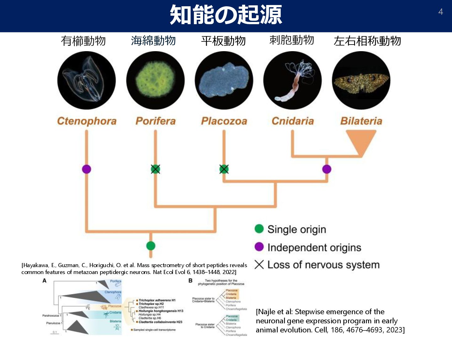
Stepwise emergence of the neuronal gene expression program in early animal evolution. Cell, 186, 4676–4693, 2023] [Hayakawa, E., Guzman, C., Horiguchi, O. et al. Mass spectrometry of short peptides reveals common features of metazoan peptidergic neurons. Nat Ecol Evol 6, 1438–1448, 2022]
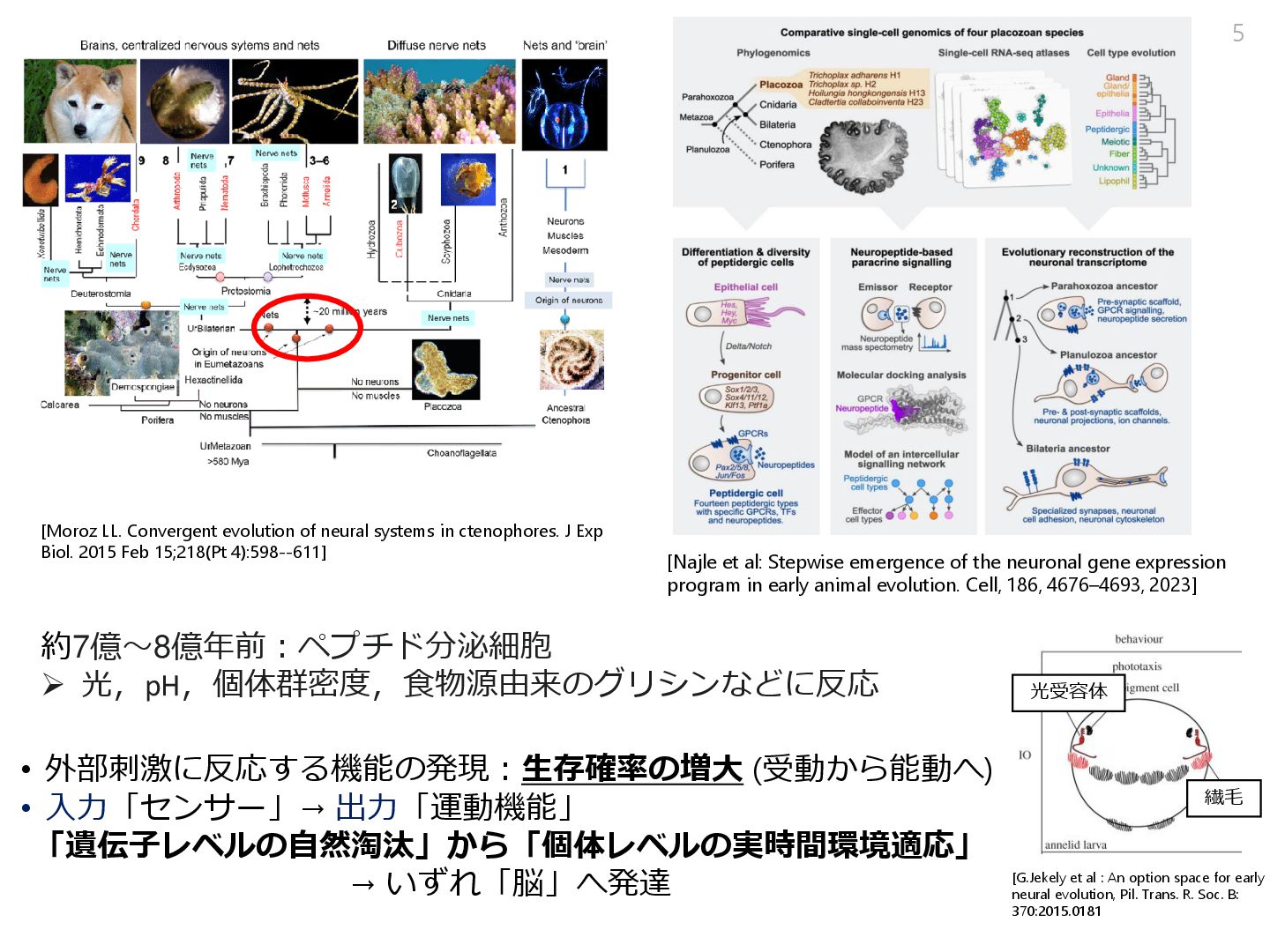
systems in ctenophores. J Exp Biol. 2015 Feb 15;218(Pt 4):598--611] [Najle et al: Stepwise emergence of the neuronal gene expression program in early animal evolution. Cell, 186, 4676–4693, 2023] • 外部刺激に反応する機能の発現:生存確率の増大 (受動から能動へ) • 入力「センサー」→ 出力「運動機能」 「遺伝子レベルの自然淘汰」から「個体レベルの実時間環境適応」 → いずれ「脳」へ発達 光受容体 繊毛 [G.Jekely et al : An option space for early neural evolution, Pil. Trans. R. Soc. B: 370:2015.0181
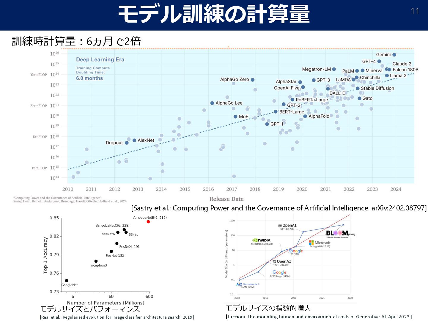
of Artificial Intelligence. arXiv:2402.08797] 訓練時計算量:6ヵ月で2倍 モデルサイズとパフォーマンス [Real et al.: Regularized evolution for image classifier architecture search. 2019] モデルサイズの指数的増大 [Luccioni. The mounting human and environmental costs of Generative AI. Apr. 2023.]
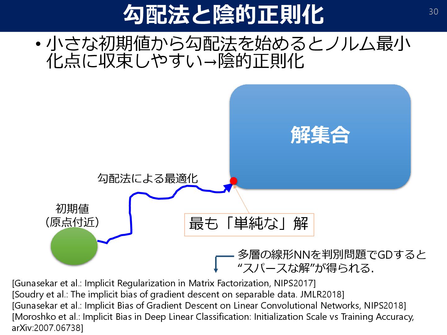
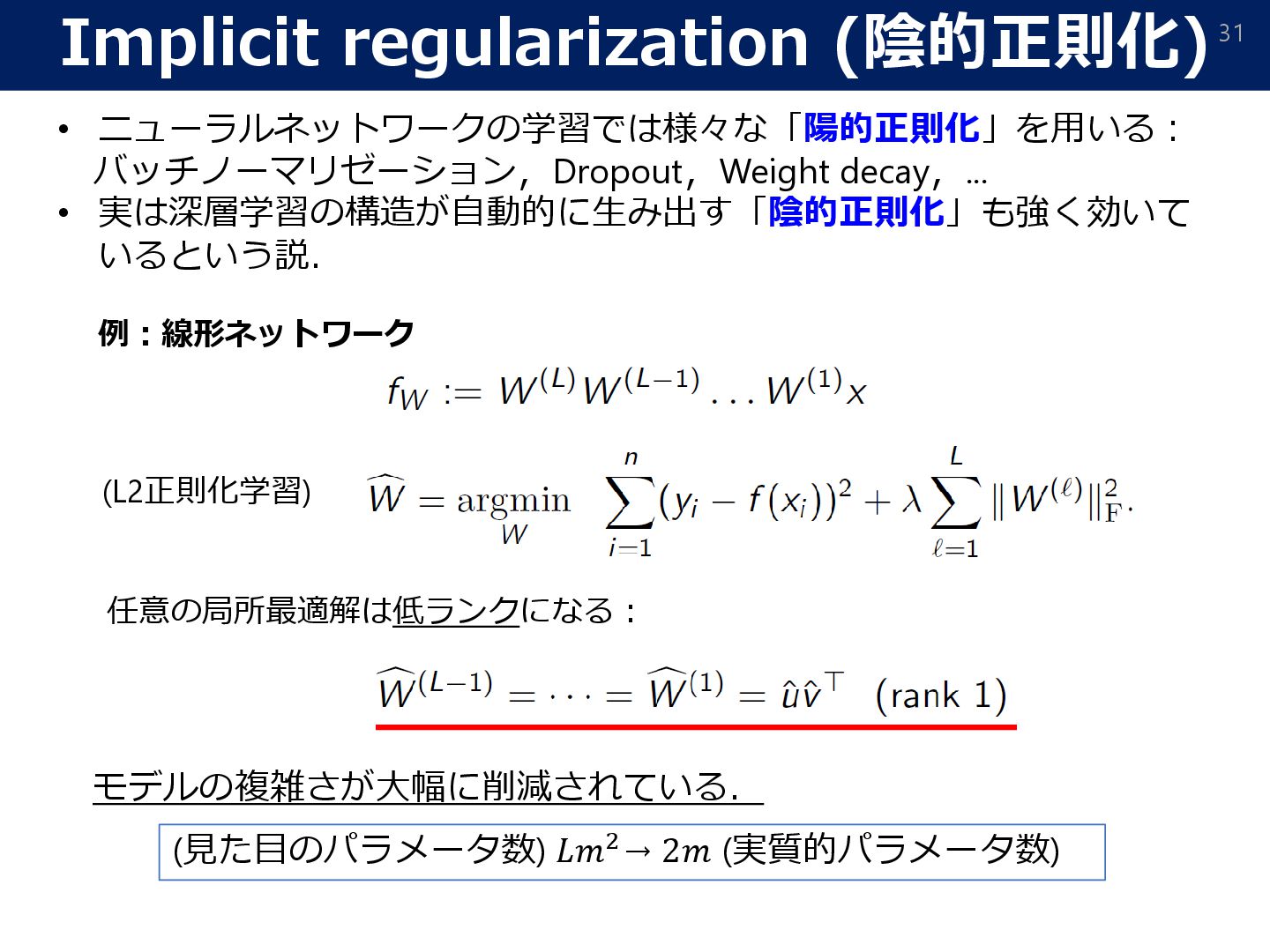
in Matrix Factorization, NIPS2017] [Soudry et al.: The implicit bias of gradient descent on separable data. JMLR2018] [Gunasekar et al.: Implicit Bias of Gradient Descent on Linear Convolutional Networks, NIPS2018] [Moroshko et al.: Implicit Bias in Deep Linear Classification: Initialization Scale vs Training Accuracy, arXiv:2007.06738] 初期値 (原点付近) 解集合 最も「単純な」解 勾配法による最適化 多層の線形NNを判別問題でGDすると “スパースな解”が得られる.
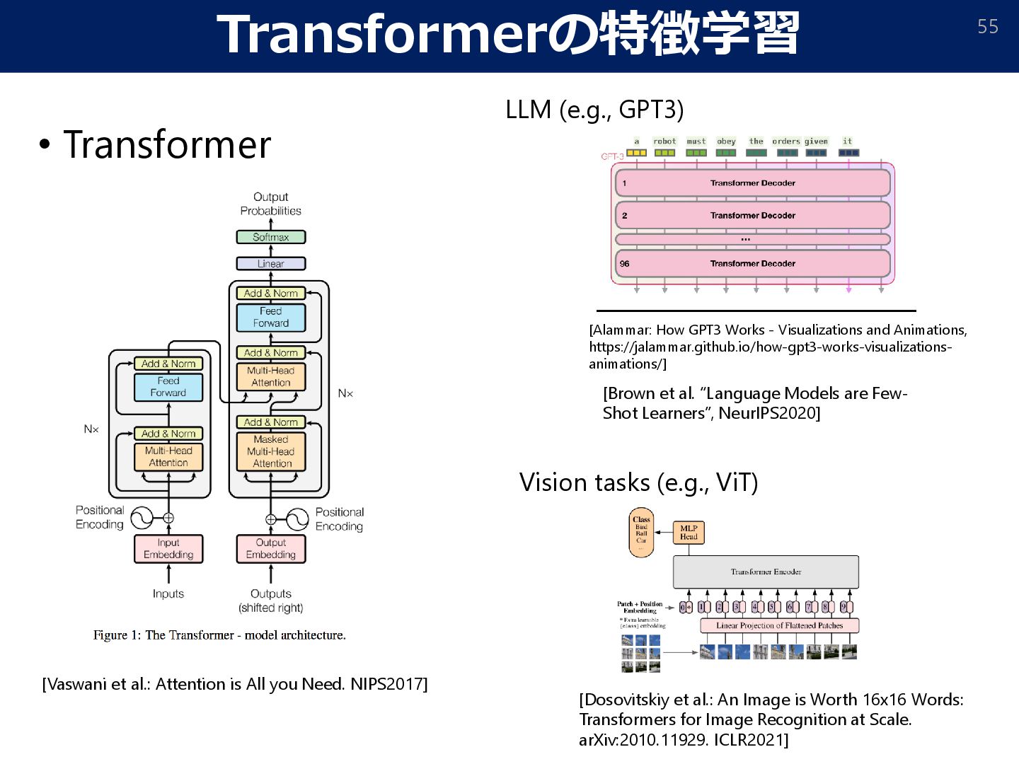
Few- Shot Learners”, NeurIPS2020] [Alammar: How GPT3 Works - Visualizations and Animations, https://jalammar.github.io/how-gpt3-works-visualizations- animations/] LLM (e.g., GPT3) [Vaswani et al.: Attention is All you Need. NIPS2017] [Dosovitskiy et al.: An Image is Worth 16x16 Words: Transformers for Image Recognition at Scale. arXiv:2010.11929. ICLR2021] Vision tasks (e.g., ViT)
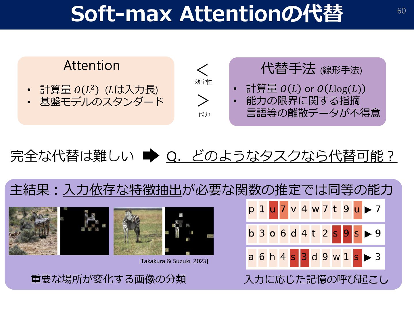
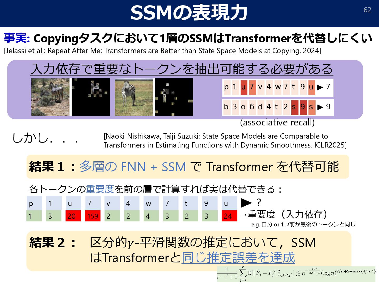
p 1 u 7 v 4 w 7 t 9 u 1 3 20 159 2 2 4 3 2 3 24 結果1:多層の FNN + SSM で Transformer を代替可能 結果2: 区分的𝛾-平滑関数の推定において,SSM はTransformerと同じ推定誤差を達成 事実: Copyingタスクにおいて1層のSSMはTransformerを代替しにくい [Jelassi et al.: Repeat After Me: Transformers are Better than State Space Models at Copying. 2024] [Naoki Nishikawa, Taiji Suzuki: State Space Models are Comparable to Transformers in Estimating Functions with Dynamic Smoothness. ICLR2025] しかし... (associative recall)
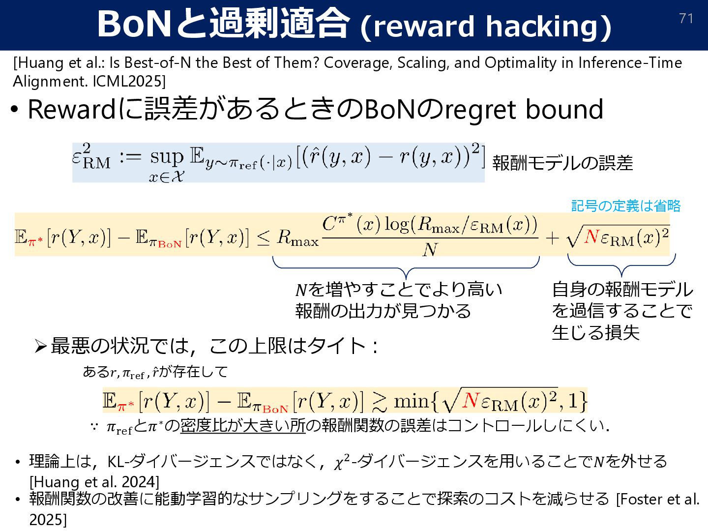
et al. 2024] • 報酬関数の改善に能動学習的なサンプリングをすることで探索のコストを減らせる [Foster et al. 2025] 記号の定義は省略 𝑁を増やすことでより高い 報酬の出力が見つかる 自身の報酬モデル を過信することで 生じる損失 ➢最悪の状況では,この上限はタイト: ある𝑟, 𝜋ref , Ƹ 𝑟が存在して ∵ 𝜋ref と𝜋∗の密度比が大きい所の報酬関数の誤差はコントロールしにくい. [Huang et al.: Is Best-of-N the Best of Them? Coverage, Scaling, and Optimality in Inference-Time Alignment. ICML2025] 報酬モデルの誤差
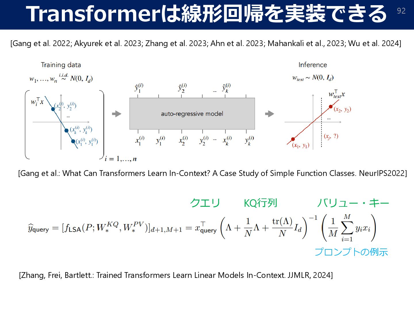
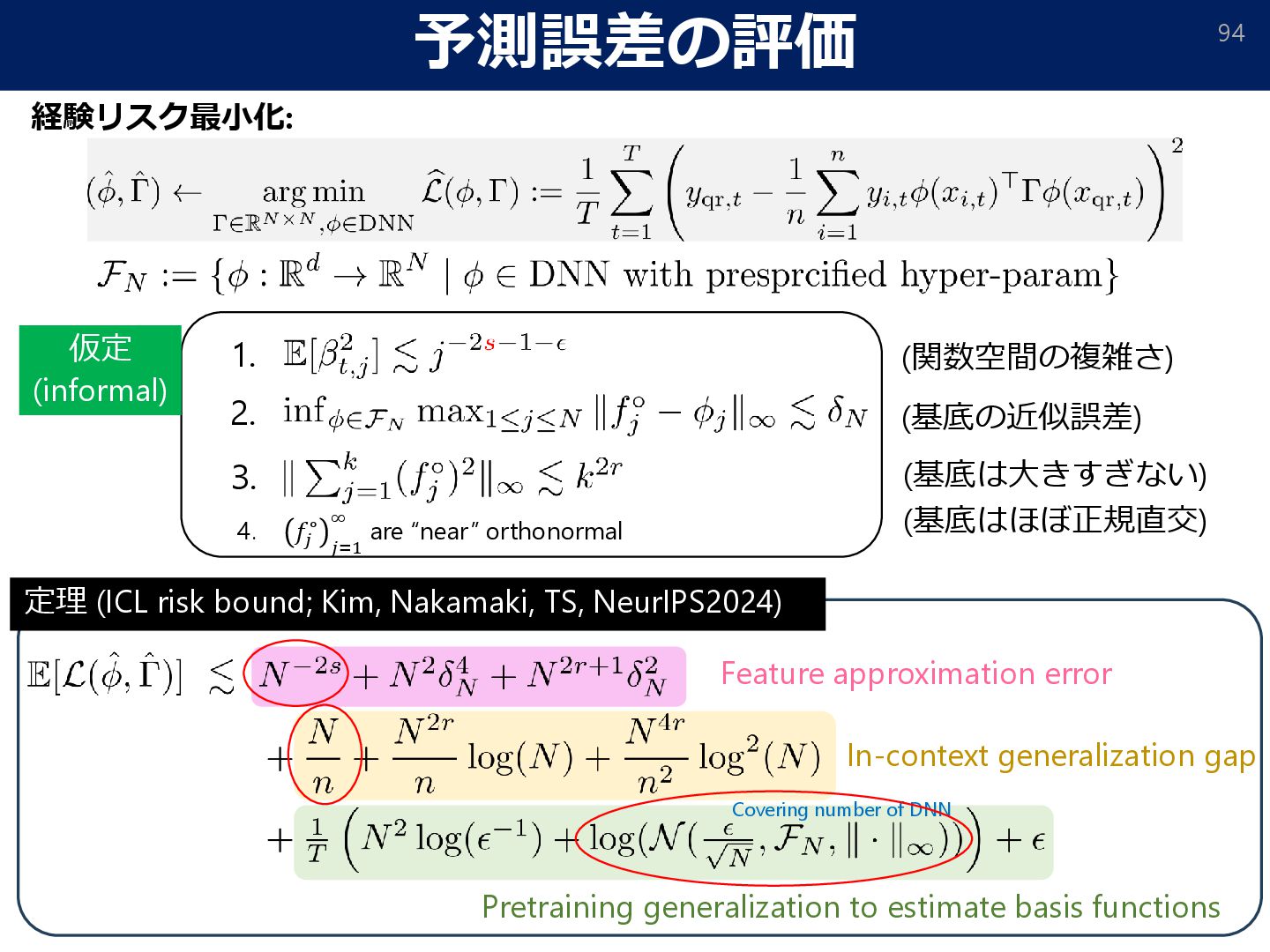
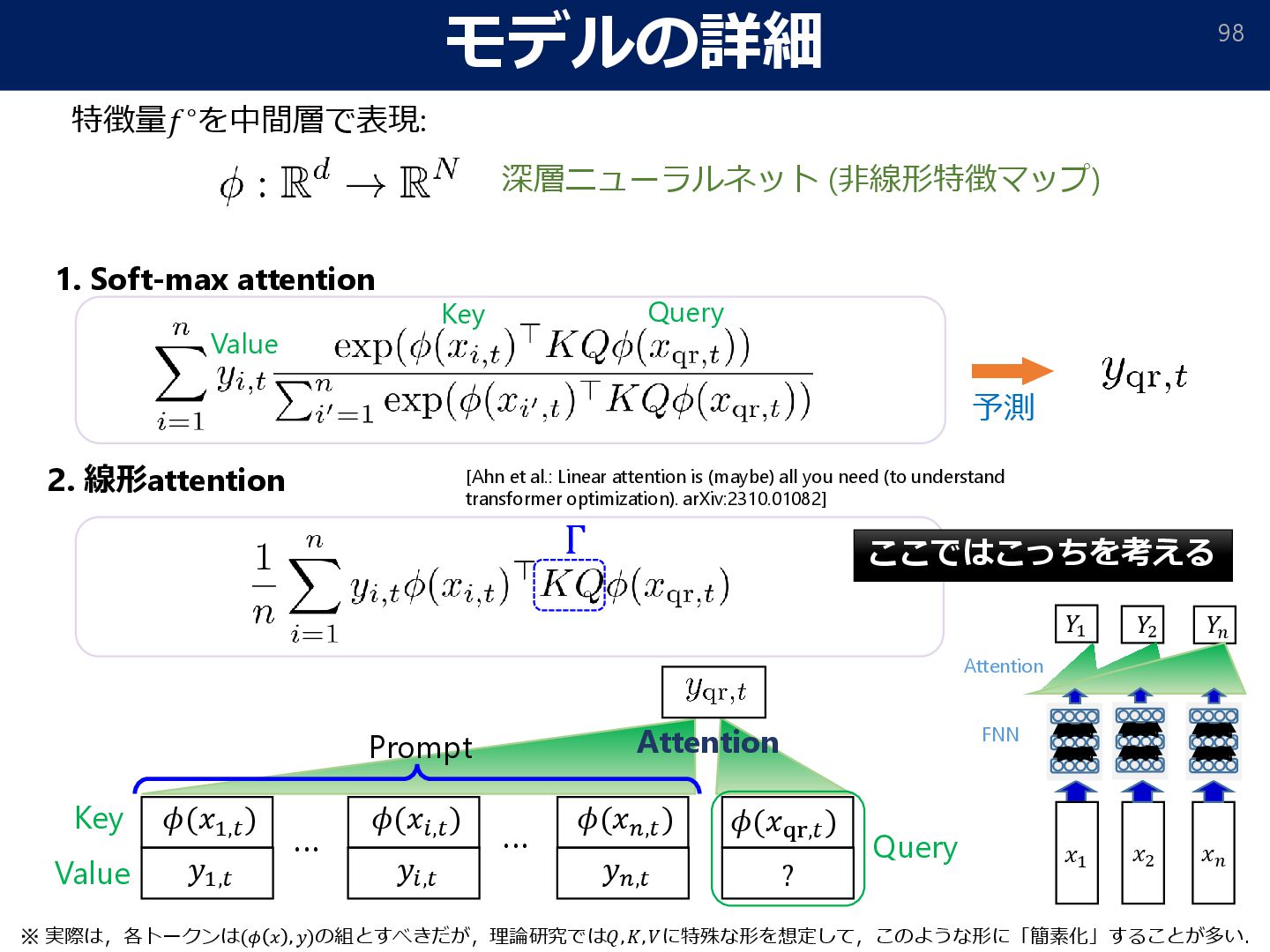
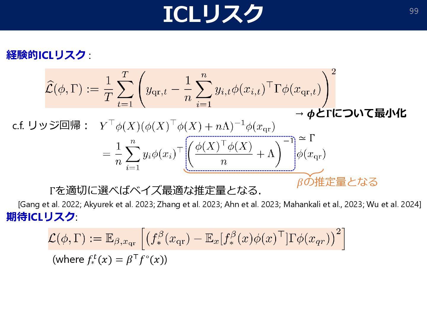
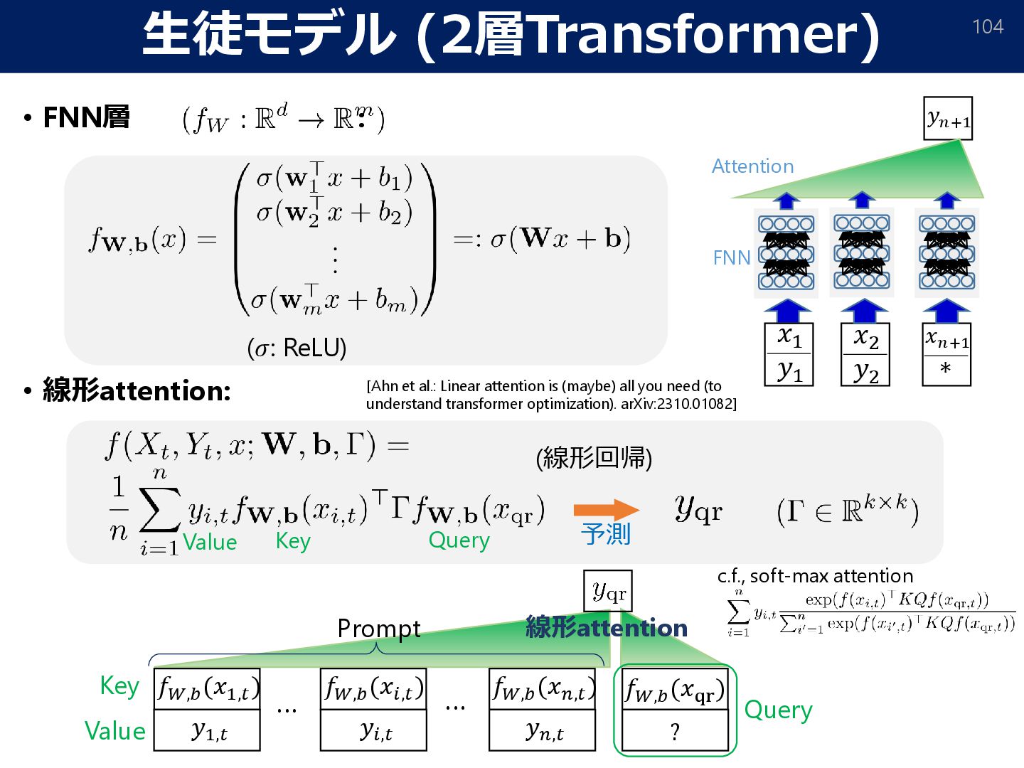
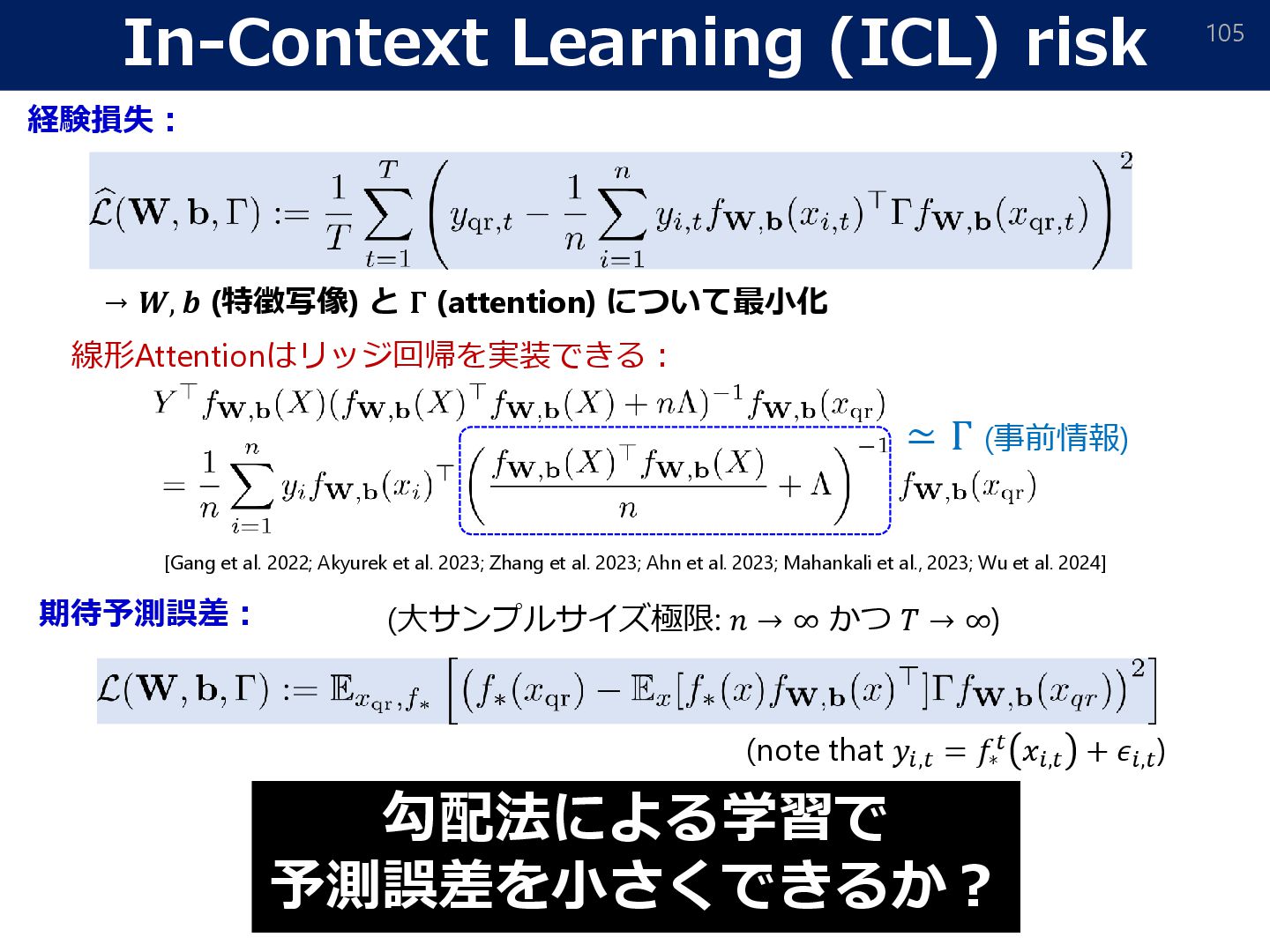
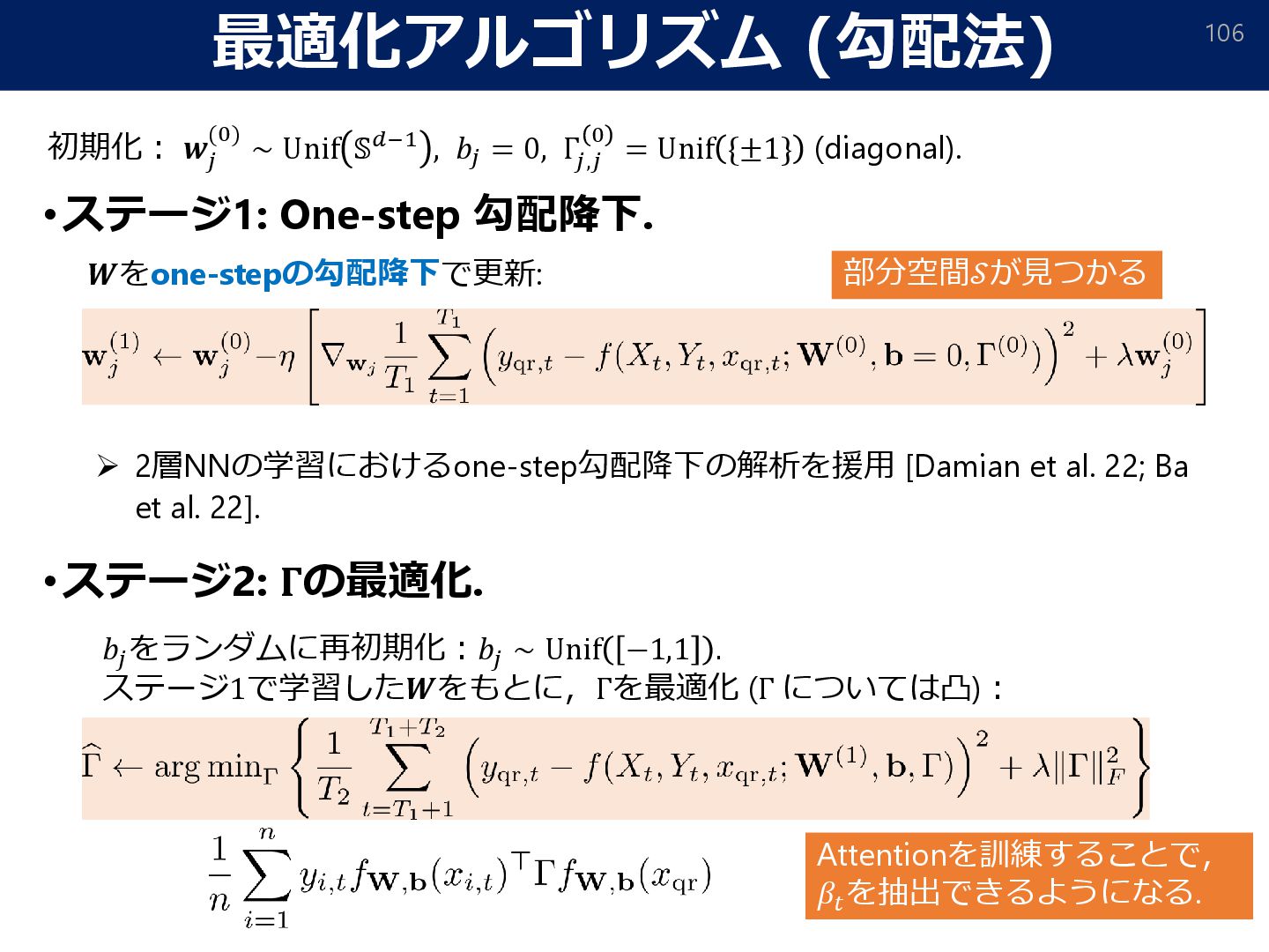
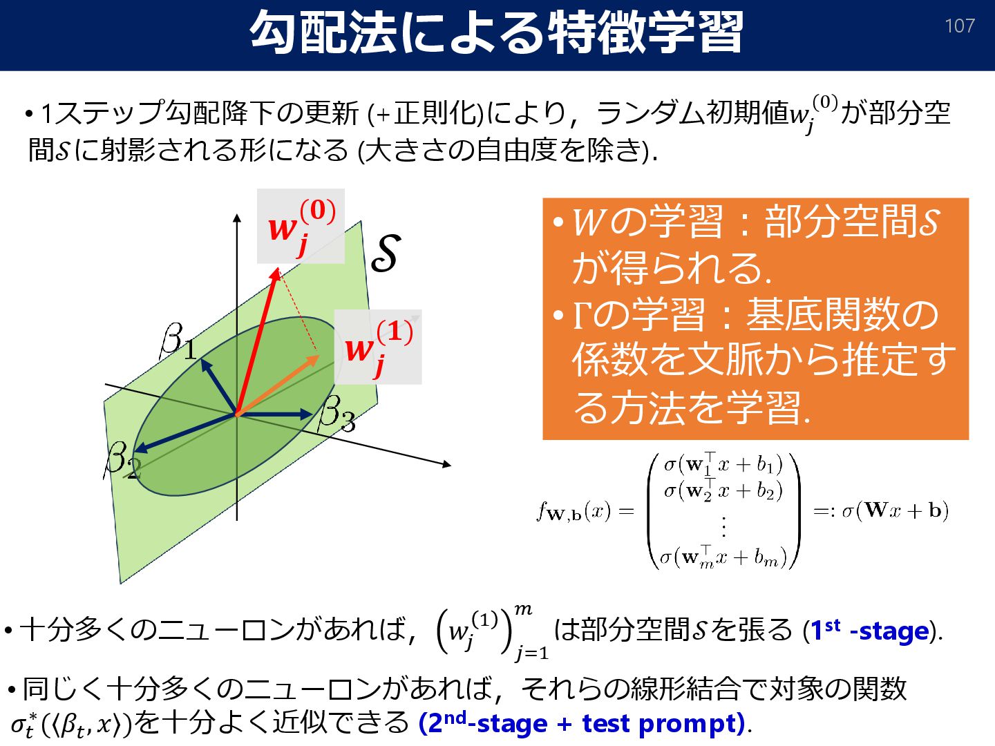
Zhang et al. 2023; Ahn et al. 2023; Mahankali et al., 2023; Wu et al. 2024] [Gang et al.: What Can Transformers Learn In-Context? A Case Study of Simple Function Classes. NeurIPS2022] [Zhang, Frei, Bartlett.: Trained Transformers Learn Linear Models In-Context. JJMLR, 2024] クエリ KQ行列 バリュー・キー プロンプトの例示
Chen, Huan Wang, Caiming Xiong, Song Mei: Transformers as Statisticians: Provable In-Context Learning with In-Context Algorithm Selection. NeurIPS2023] ✓ 実際には,浅い層で特徴抽出をし,深い層で勾配法を実行しているらしい [Guo et al., 2023; von Oswald et al., 2023].
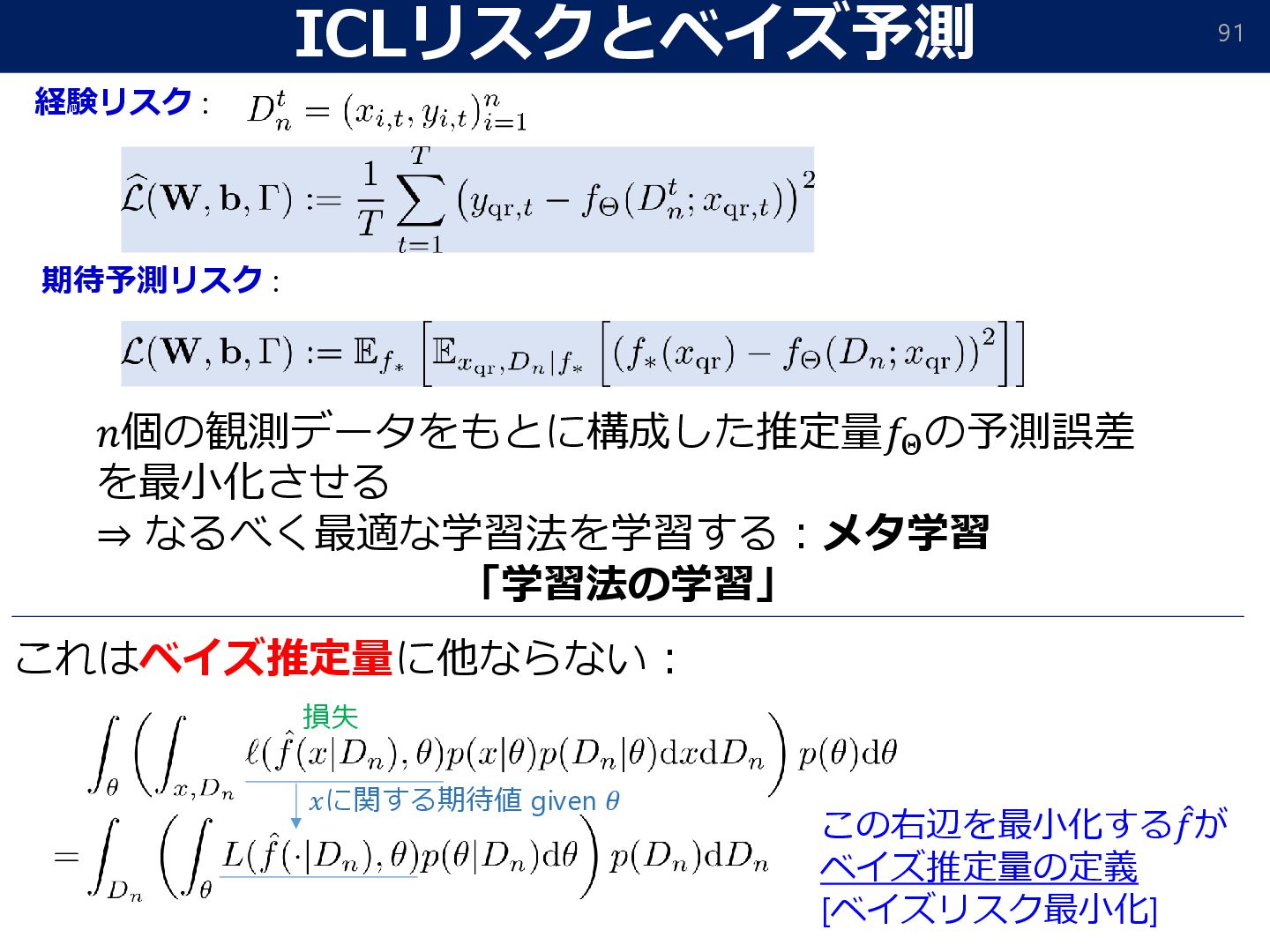
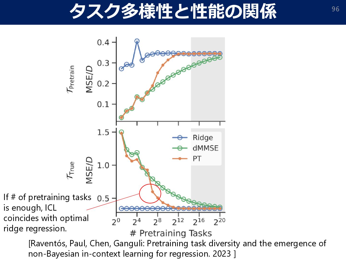
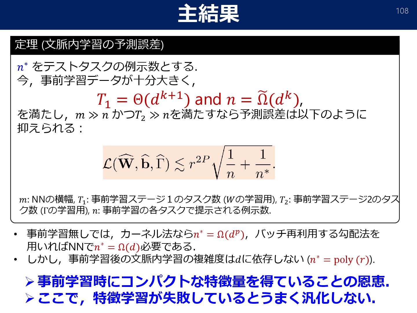
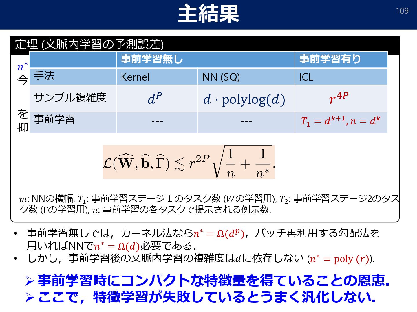
the emergence of non-Bayesian in-context learning for regression. 2023 ] If # of pretraining tasks is enough, ICL coincides with optimal ridge regression.
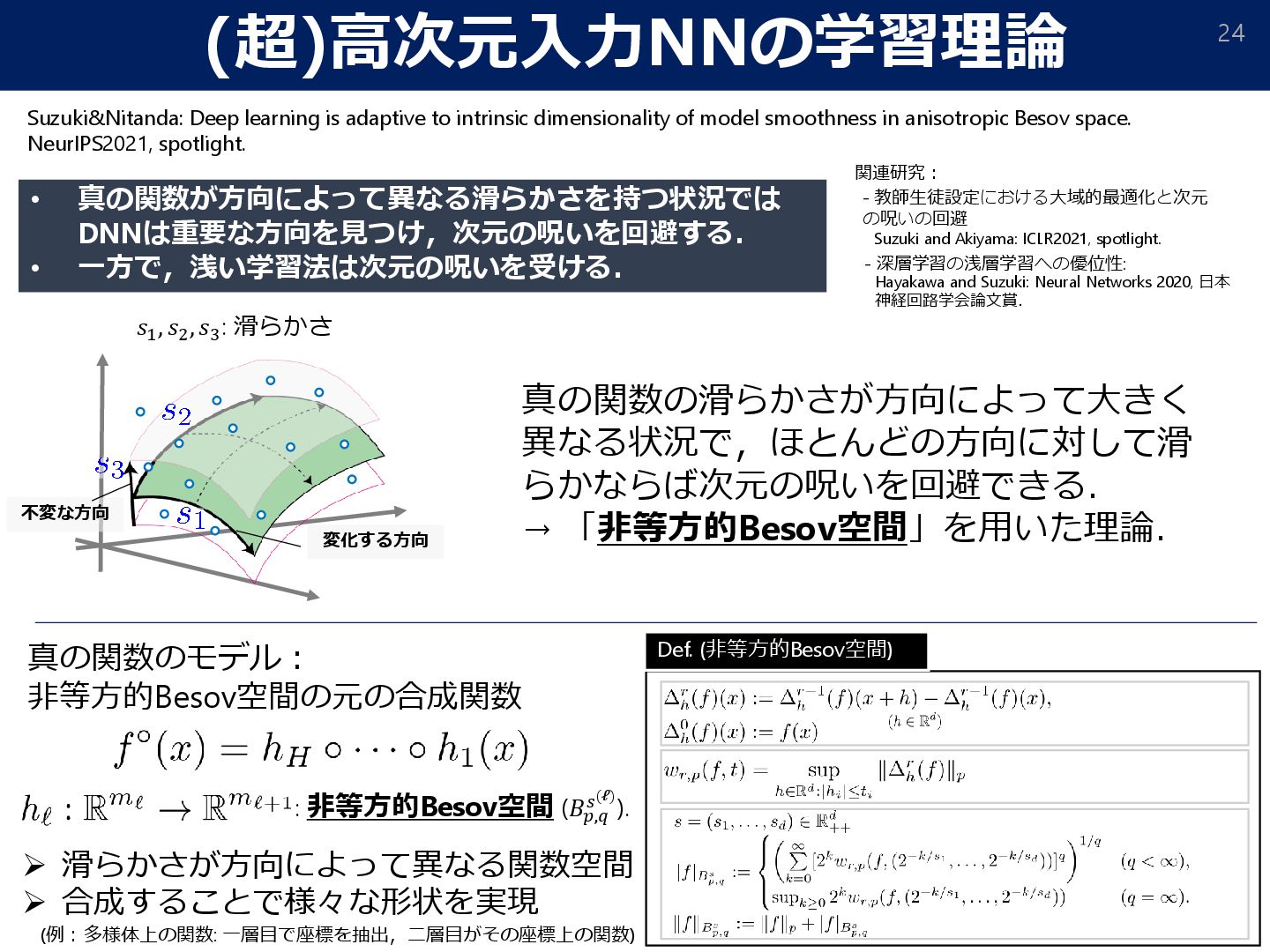
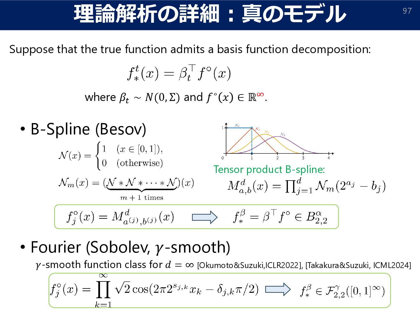
∈ ℝ∞. Suppose that the true function admits a basis function decomposition: • B-Spline (Besov) • Fourier (Sobolev, 𝛾-smooth) Tensor product B-spline: 𝛾-smooth function class for 𝑑 = ∞ [Okumoto&Suzuki,ICLR2022], [Takakura&Suzuki, ICML2024]
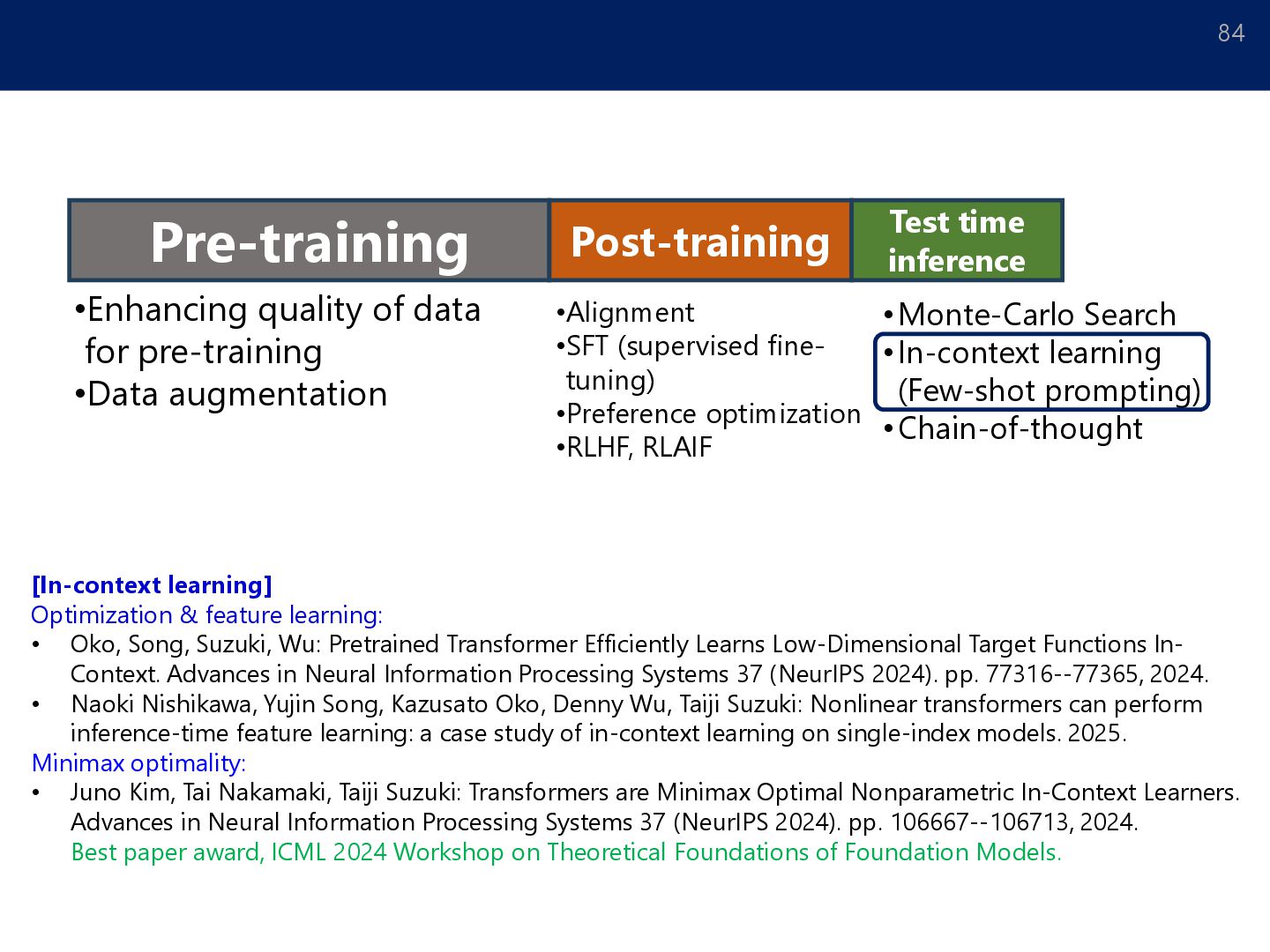
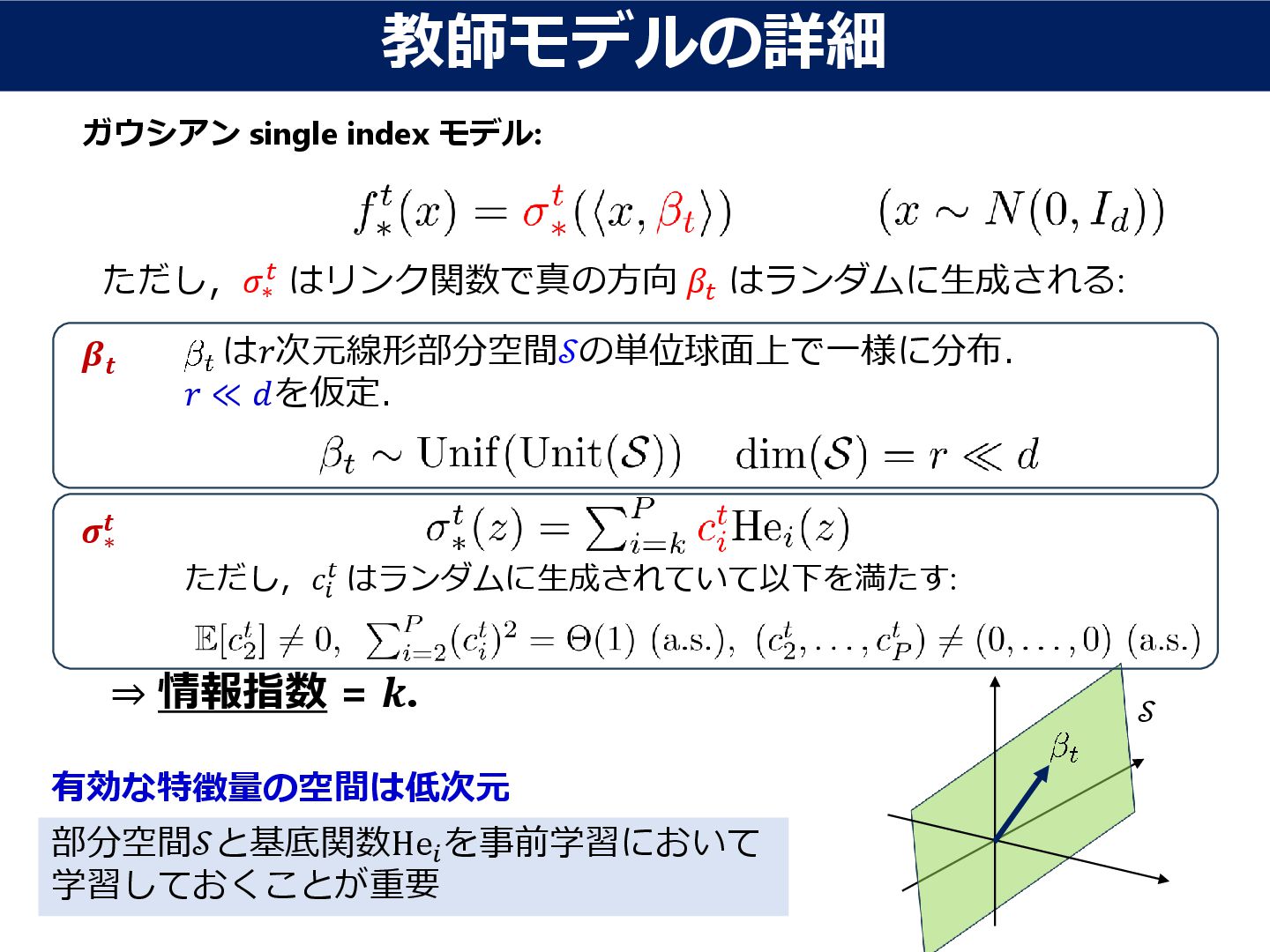
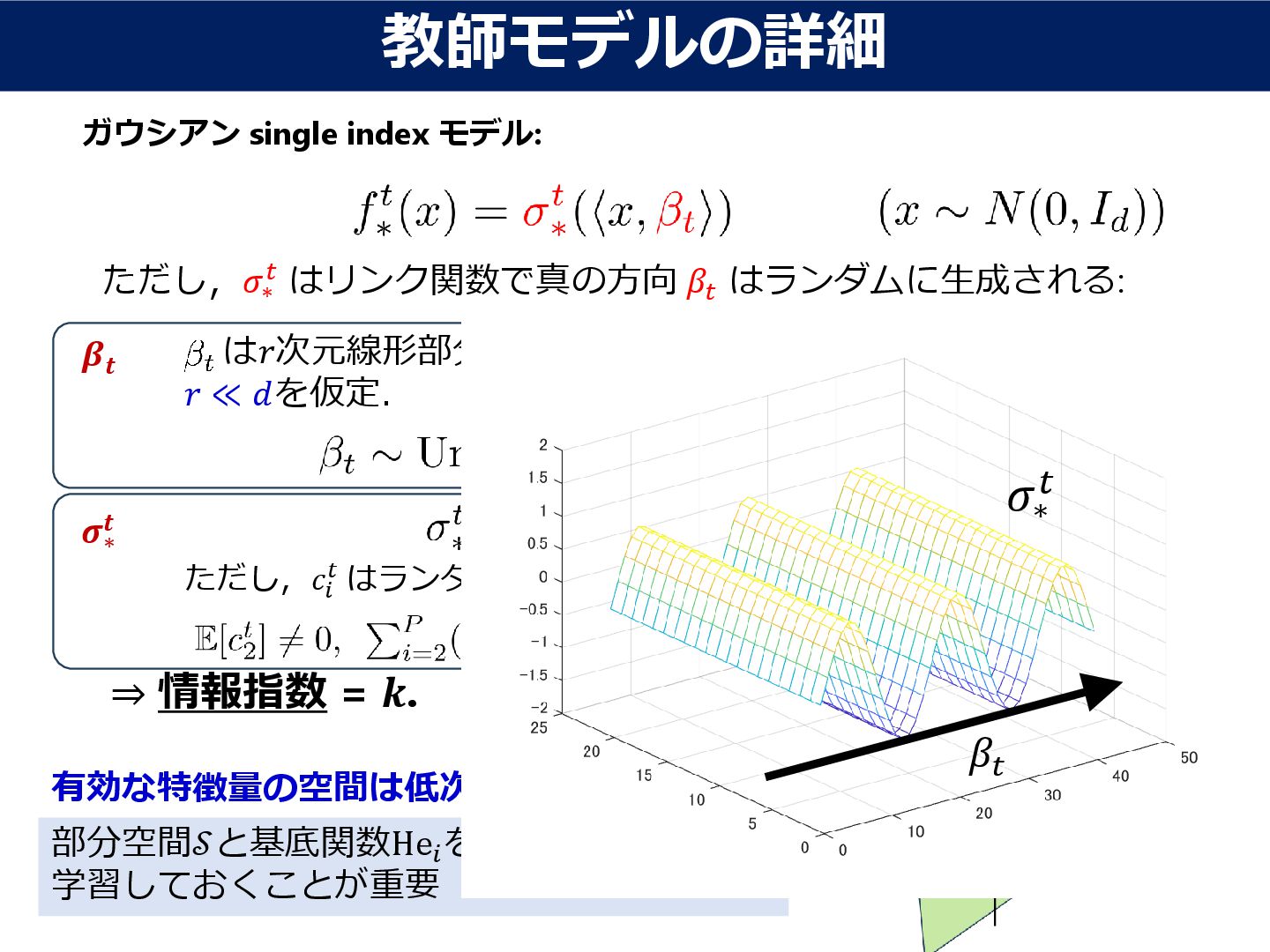
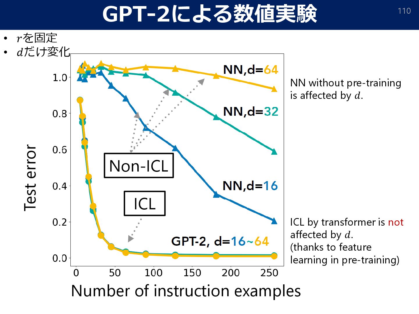
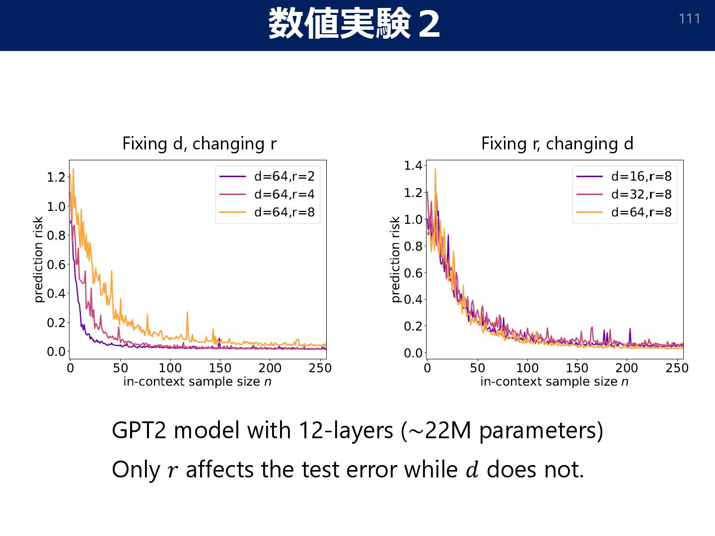
Wu: Pretrained Transformer Efficiently Learns Low-Dimensional Target Functions In- Context. Advances in Neural Information Processing Systems 37 (NeurIPS 2024). pp. 77316--77365, 2024. • Naoki Nishikawa, Yujin Song, Kazusato Oko, Denny Wu, Taiji Suzuki: Nonlinear transformers can perform inference-time feature learning: a case study of in-context learning on single-index models. ICML2025.
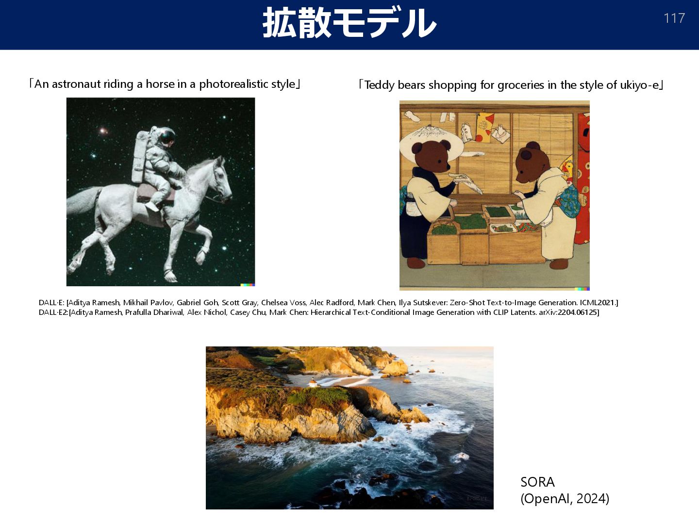
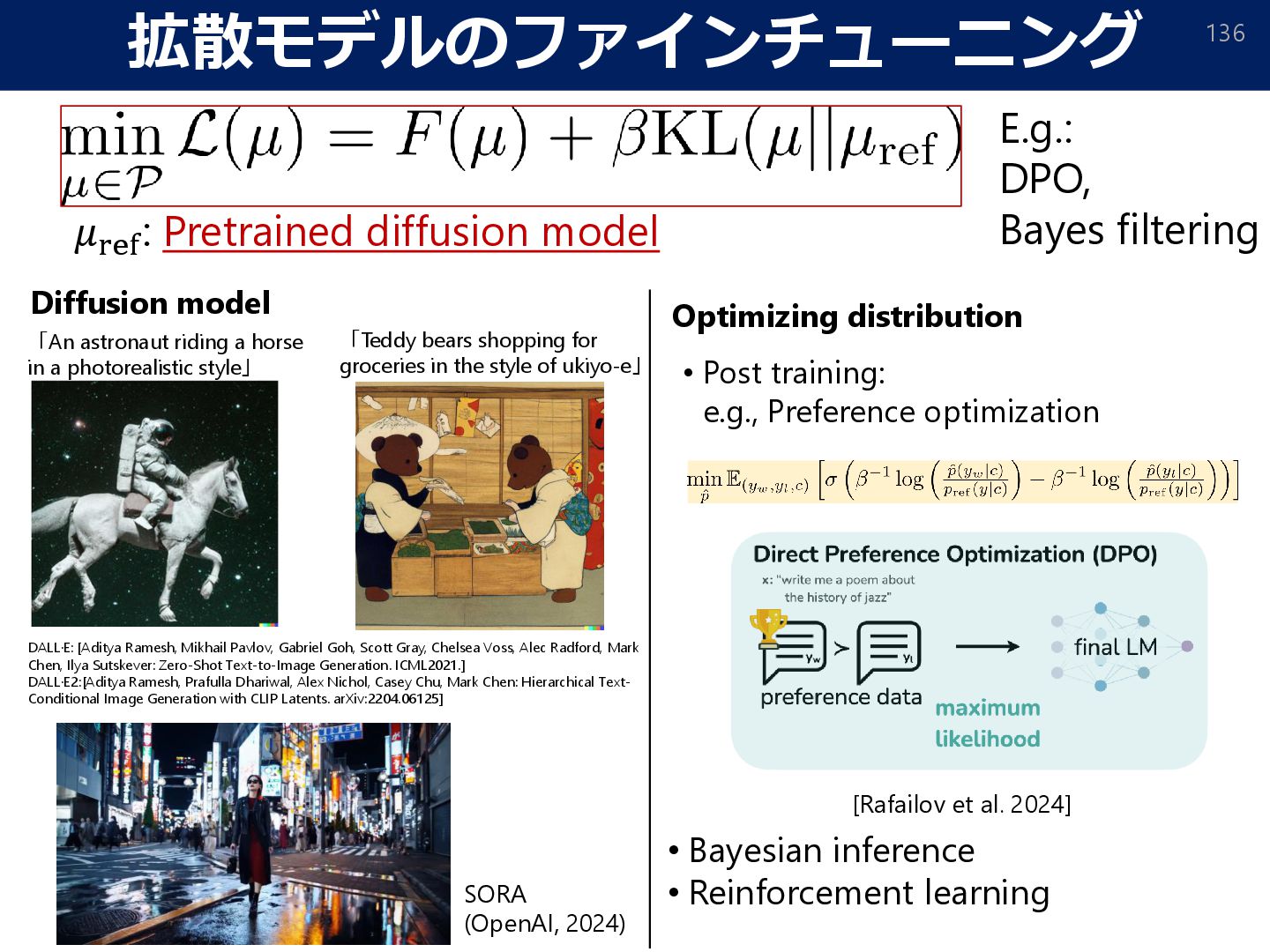
style」 「Teddy bears shopping for groceries in the style of ukiyo-e」 SORA (OpenAI, 2024) DALL·E: [Aditya Ramesh, Mikhail Pavlov, Gabriel Goh, Scott Gray, Chelsea Voss, Alec Radford, Mark Chen, Ilya Sutskever: Zero-Shot Text-to-Image Generation. ICML2021.] DALL·E2:[Aditya Ramesh, Prafulla Dhariwal, Alex Nichol, Casey Chu, Mark Chen: Hierarchical Text-Conditional Image Generation with CLIP Latents. arXiv:2204.06125]
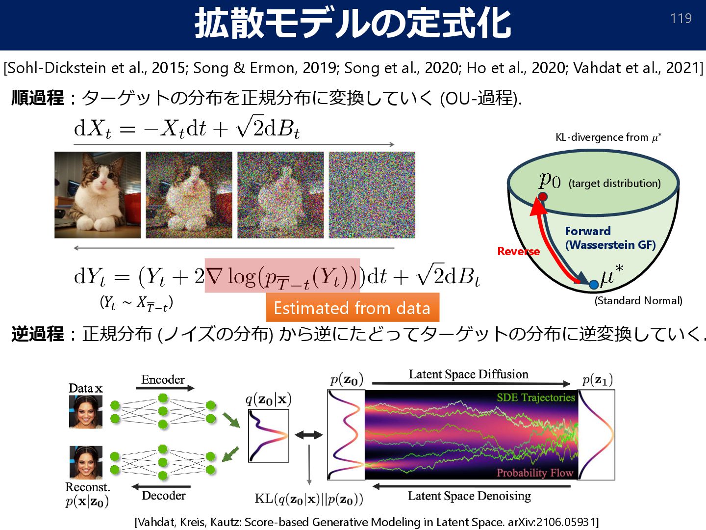
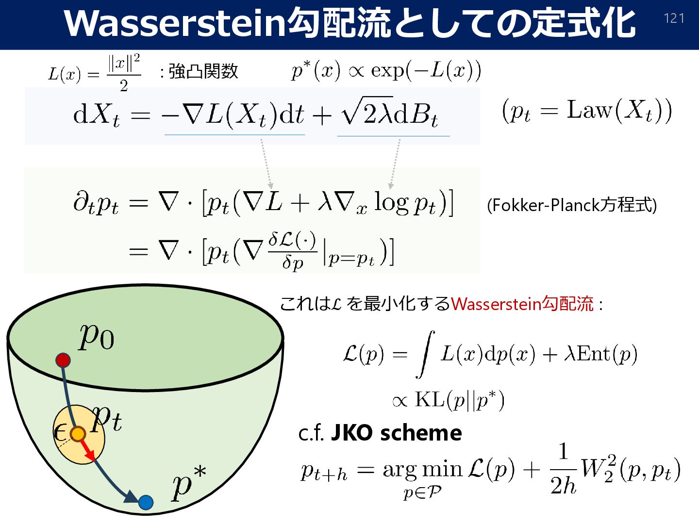
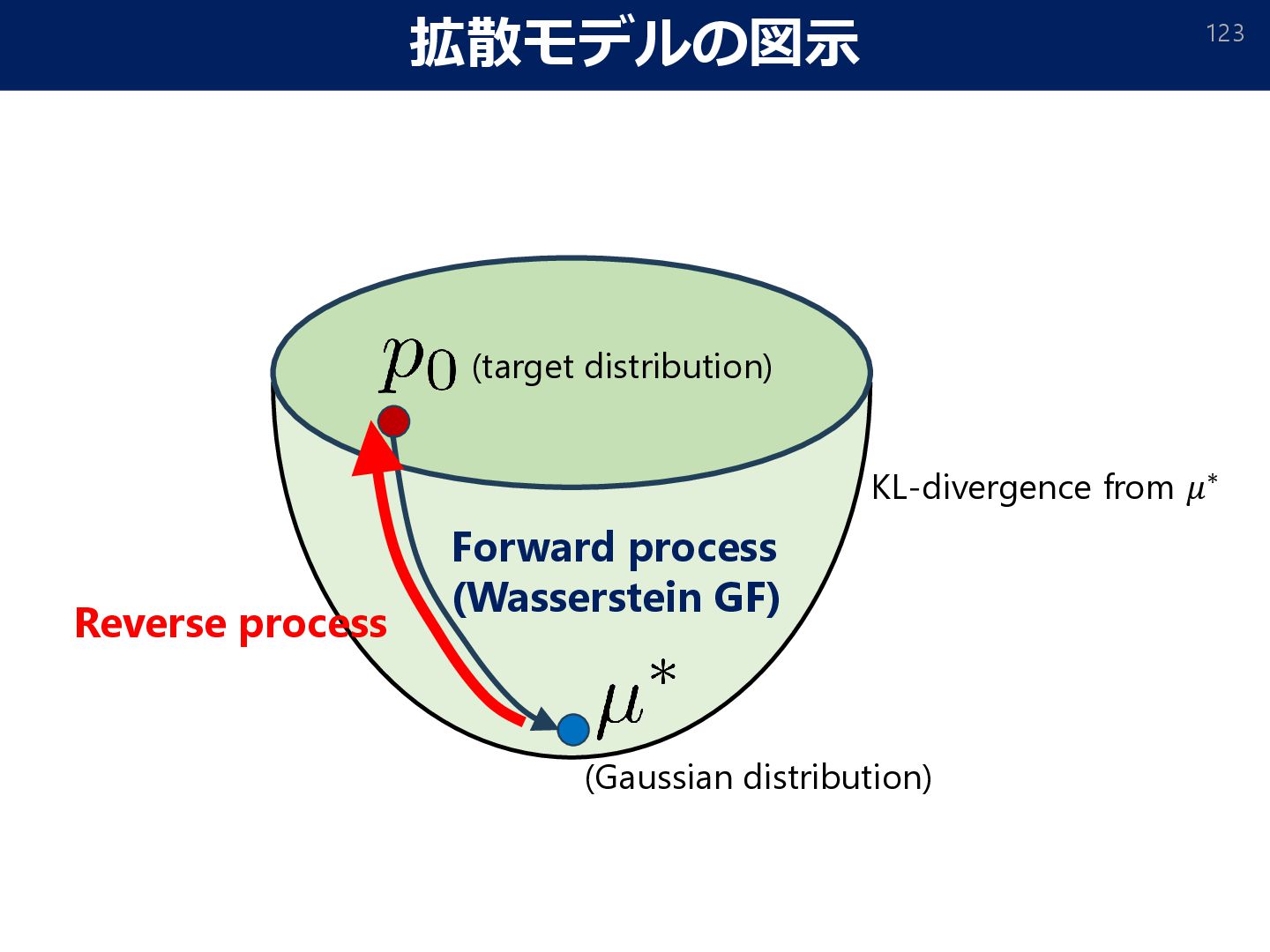
Score-based Generative Modeling in Latent Space. arXiv:2106.05931] (𝑌𝑡 ∼ 𝑋 𝑇−𝑡 ) [Sohl-Dickstein et al., 2015; Song & Ermon, 2019; Song et al., 2020; Ho et al., 2020; Vahdat et al., 2021] Estimated from data Reverse (target distribution) (Standard Normal) Forward (Wasserstein GF) KL-divergence from 𝜇∗
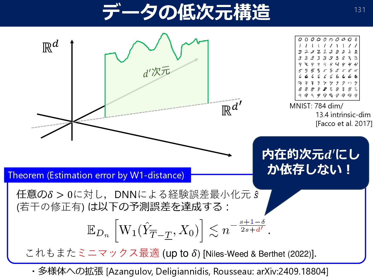
129 Assumption 1 The true distribution 𝑝0 is supported on −1,1 𝑑 and with 𝑠 > Τ 1 𝑝 − Τ 1 2 + as a density function on −1,1 𝑑. Assumption2 Very smooth Besov space Besov space (𝐵𝑝,𝑞 𝑠 (Ω)) Smoothness Spatial inhomogeneity Reference
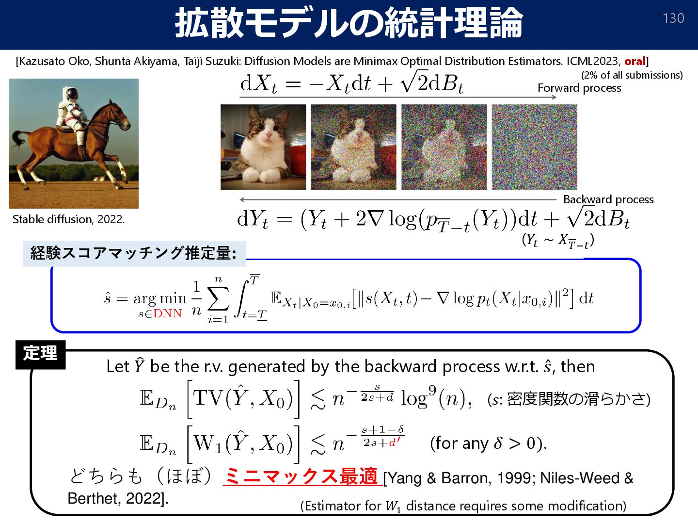
Forward process Backward process どちらも(ほぼ)ミニマックス最適 [Yang & Barron, 1999; Niles-Weed & Berthet, 2022]. 経験スコアマッチング推定量: (for any 𝛿 > 0). 定理 Let 𝑌 be the r.v. generated by the backward process w.r.t. Ƹ 𝑠, then (Estimator for 𝑊1 distance requires some modification) (𝑠: 密度関数の滑らかさ) [Kazusato Oko, Shunta Akiyama, Taiji Suzuki: Diffusion Models are Minimax Optimal Distribution Estimators. ICML2023, oral] (2% of all submissions)
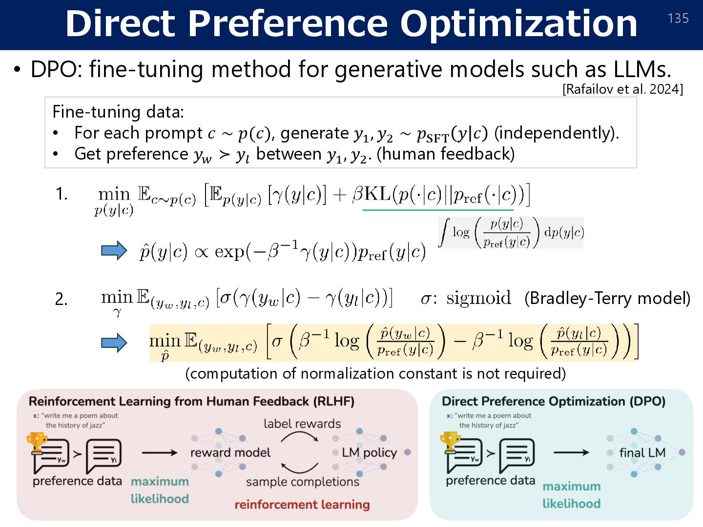
such as LLMs. 135 Fine-tuning data: • For each prompt 𝑐 ∼ 𝑝(𝑐), generate 𝑦1 , 𝑦2 ∼ 𝑝SFT 𝑦 𝑐 (independently). • Get preference 𝑦𝑤 ≻ 𝑦𝑙 between 𝑦1 , 𝑦2. (human feedback) 1. 2. (Bradley-Terry model) (computation of normalization constant is not required) [Rafailov et al. 2024]
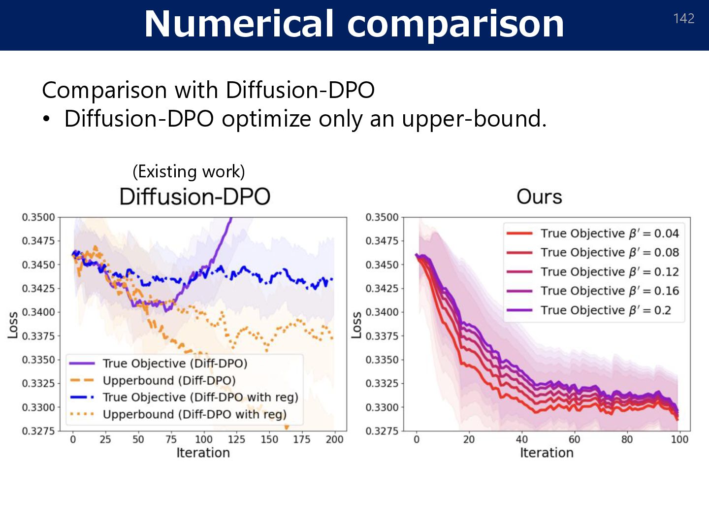
style」 「Teddy bears shopping for groceries in the style of ukiyo-e」 SORA (OpenAI, 2024) Diffusion model DALL·E: [Aditya Ramesh, Mikhail Pavlov, Gabriel Goh, Scott Gray, Chelsea Voss, Alec Radford, Mark Chen, Ilya Sutskever: Zero-Shot Text-to-Image Generation. ICML2021.] DALL·E2:[Aditya Ramesh, Prafulla Dhariwal, Alex Nichol, Casey Chu, Mark Chen: Hierarchical Text- Conditional Image Generation with CLIP Latents. arXiv:2204.06125] Optimizing distribution [Rafailov et al. 2024] • Post training: e.g., Preference optimization • Bayesian inference • Reinforcement learning E.g.: DPO, Bayes filtering 𝜇ref: Pretrained diffusion model
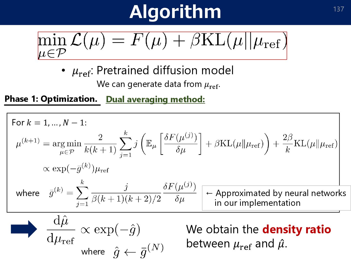
Algorithm 137 We can generate data from 𝜇ref. Dual averaging method: • 𝜇ref: Pretrained diffusion model where For 𝑘 = 1, … , 𝑁 − 1: Phase 1: Optimization. where ← Approximated by neural networks in our implementation
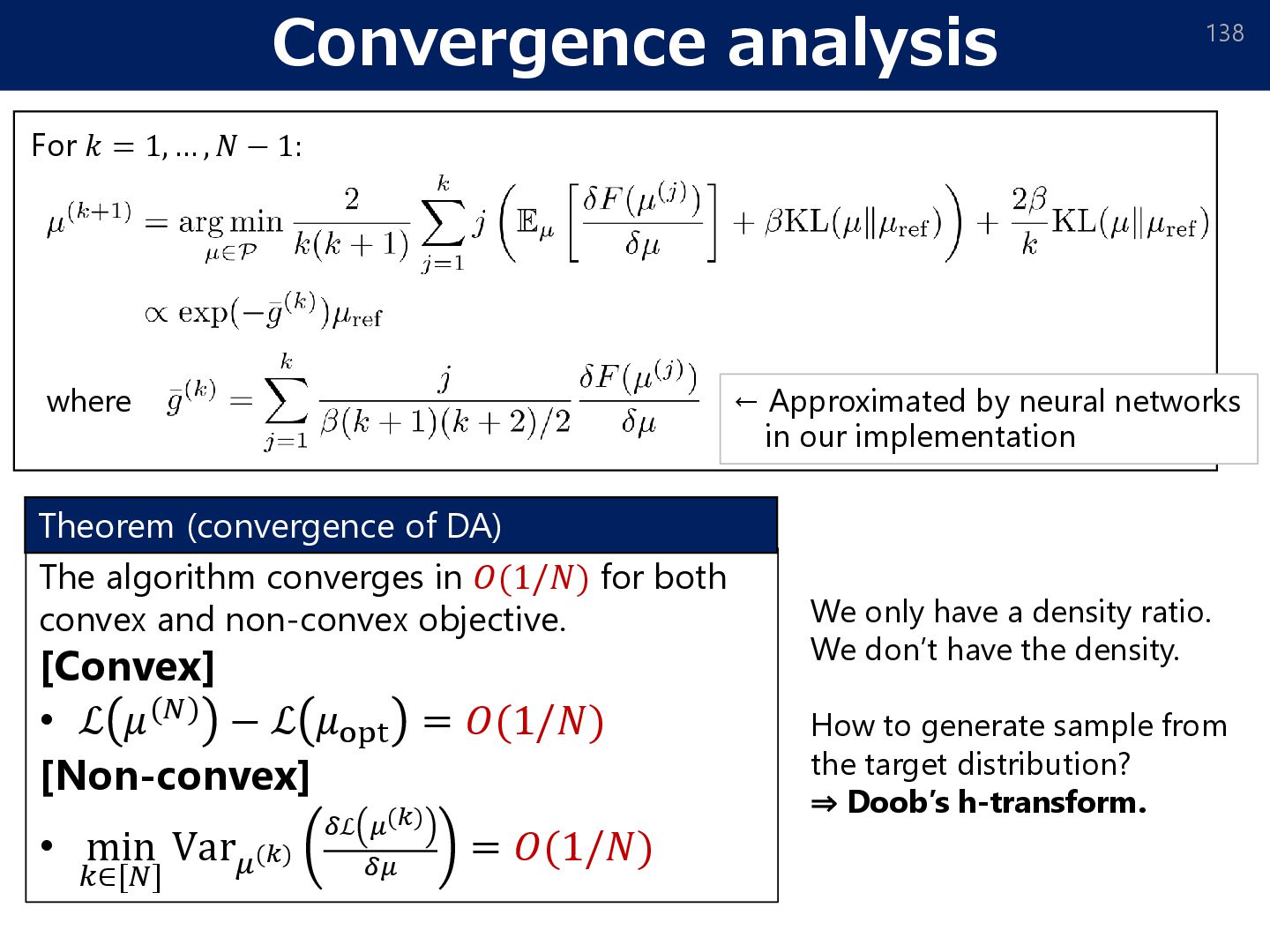
𝑁 − 1: ← Approximated by neural networks in our implementation The algorithm converges in 𝑂(1/𝑁) for both convex and non-convex objective. [Convex] • ℒ 𝜇(𝑁) − ℒ 𝜇opt = 𝑂(1/𝑁) [Non-convex] • min 𝑘∈[𝑁] Var 𝜇(𝑘) 𝛿ℒ 𝜇(𝑘) 𝛿𝜇 = 𝑂(1/𝑁) Theorem (convergence of DA) We only have a density ratio. We don’t have the density. How to generate sample from the target distribution? ⇒ Doob’s h-transform.
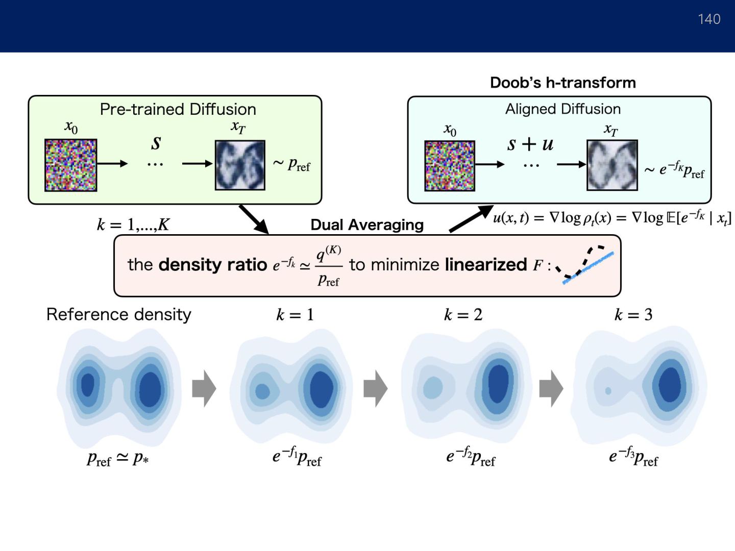
𝐞𝐱𝐩(−ෝ 𝒈) 𝝁𝐫𝐞𝐟. Doob ℎ-Transform (Doob, 1957; Rogers & Williams, 2000) Correction term Reverse process for reference model Reference model (Gaussian distribution) Corrected process Optimal model Correction reference (𝜇ref) Corrected process Ƹ 𝜇 𝑌0 𝑌ത 𝑇 𝜇ref Reverse process of 𝜇ref: See also Vargas, Grathwohl, Doucet (2023) & Heng, De Bortoli, Doucet (2024), Uehara et al. (2024) for more details.
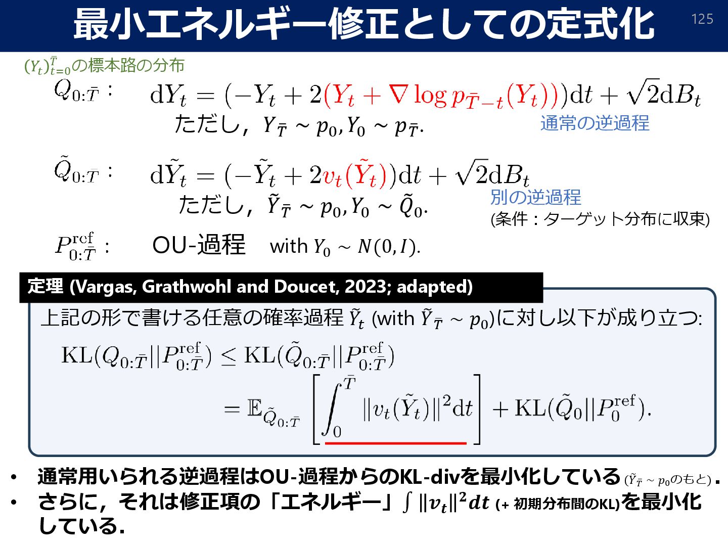
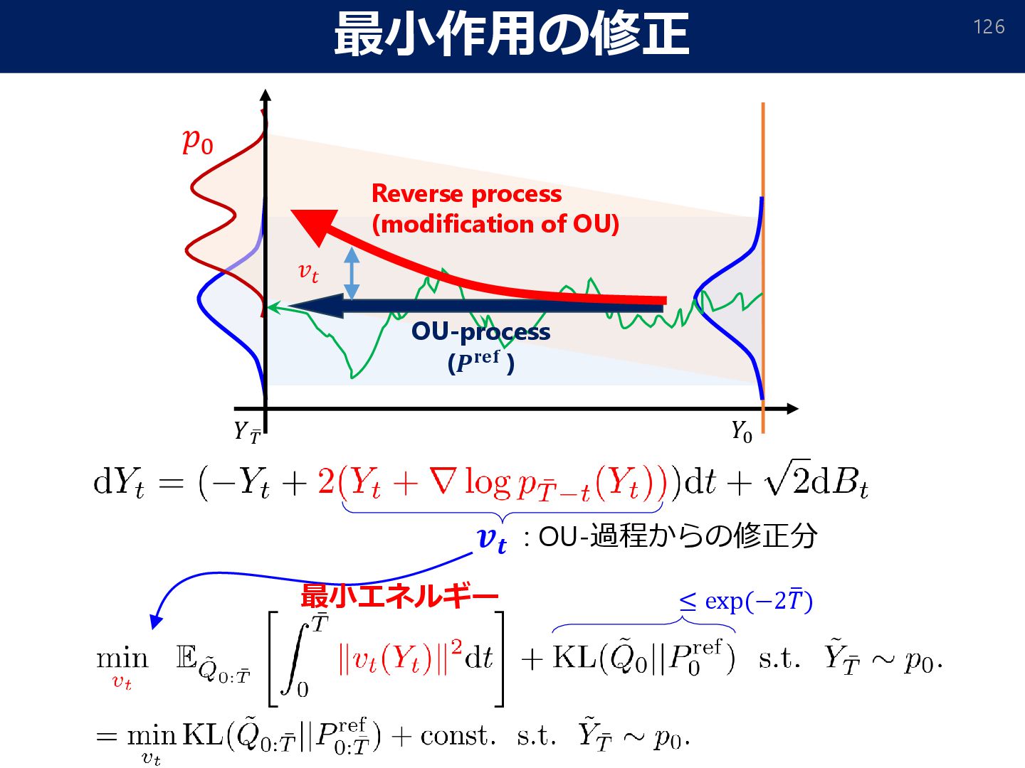
෨ 𝑌ത 𝑇 ∼ ො 𝜇, 𝑌0 ∼ 𝑝init. with 𝑌0 ∼ 𝑃0 ref. Theorem (Vargas, Grathwohl and Doucet, 2023; adapted) The doob h-transform can be characterized by “minimum energy” ∫ 𝒗𝒕 𝟐𝒅𝒕 solution. (+ KL between initial distributions). For any process ෨ 𝑌𝑡 with ෨ 𝑌ത 𝑇 ∼ ො 𝜇, it holds that (Both process converge to the target distribution) Path measure of 𝑌𝑡 𝑡=0 ത 𝑇 ∵ the construction of ℎ-transform
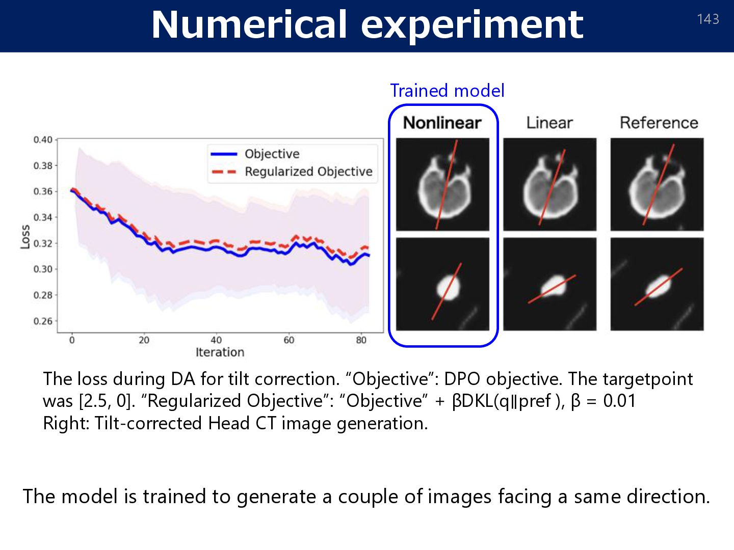
couple of images facing a same direction. The loss during DA for tilt correction. “Objective”: DPO objective. The targetpoint was [2.5, 0]. “Regularized Objective”: “Objective” + βDKL(q∥pref ), β = 0.01 Right: Tilt-corrected Head CT image generation. Trained model
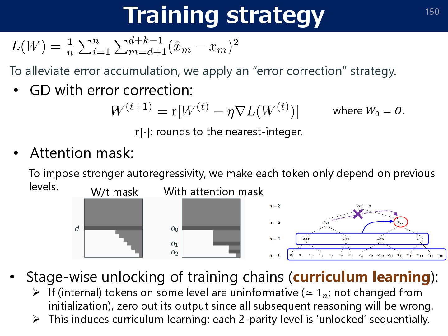
= 𝑂. r[⋅]: rounds to the nearest-integer. To alleviate error accumulation, we apply an “error correction” strategy. • Attention mask: To impose stronger autoregressivity, we make each token only depend on previous levels. W/t mask With attention mask • Stage-wise unlocking of training chains (curriculum learning): ➢ If (internal) tokens on some level are uninformative (≃ 1𝑛; not changed from initialization), zero out its output since all subsequent reasoning will be wrong. ➢ This induces curriculum learning: each 2-parity level is ‘unlocked’ sequentially.
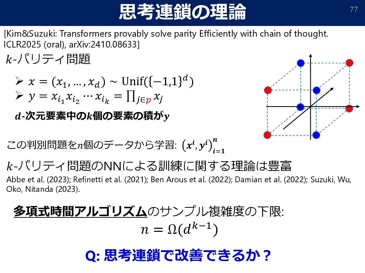
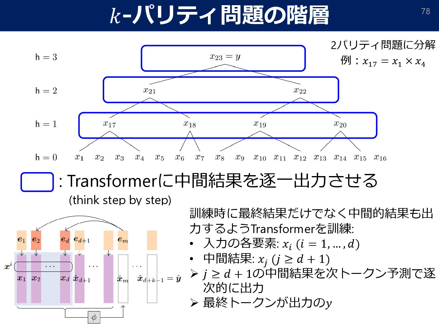
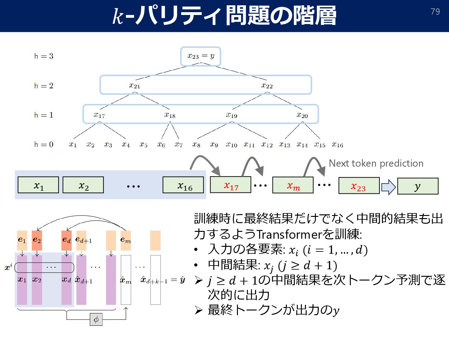
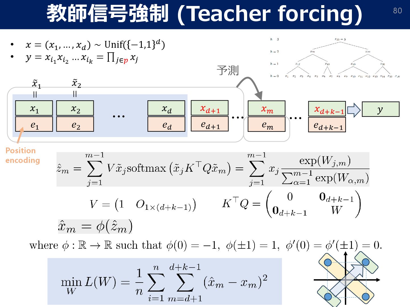
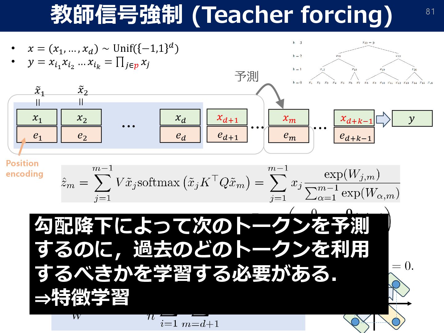
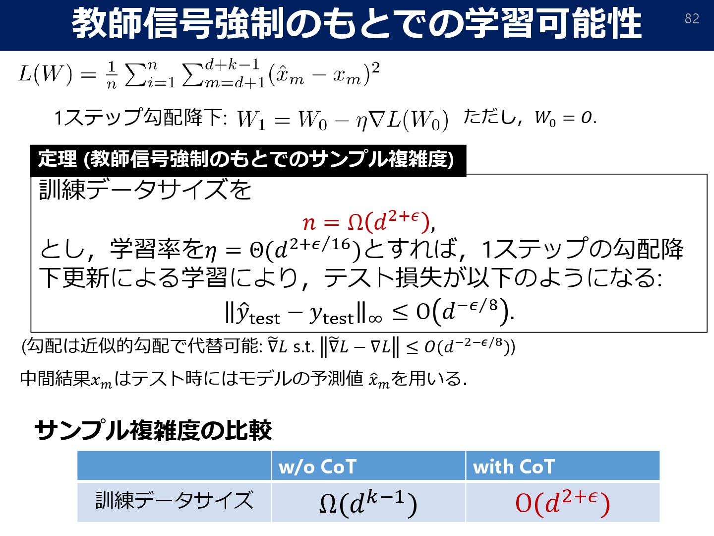
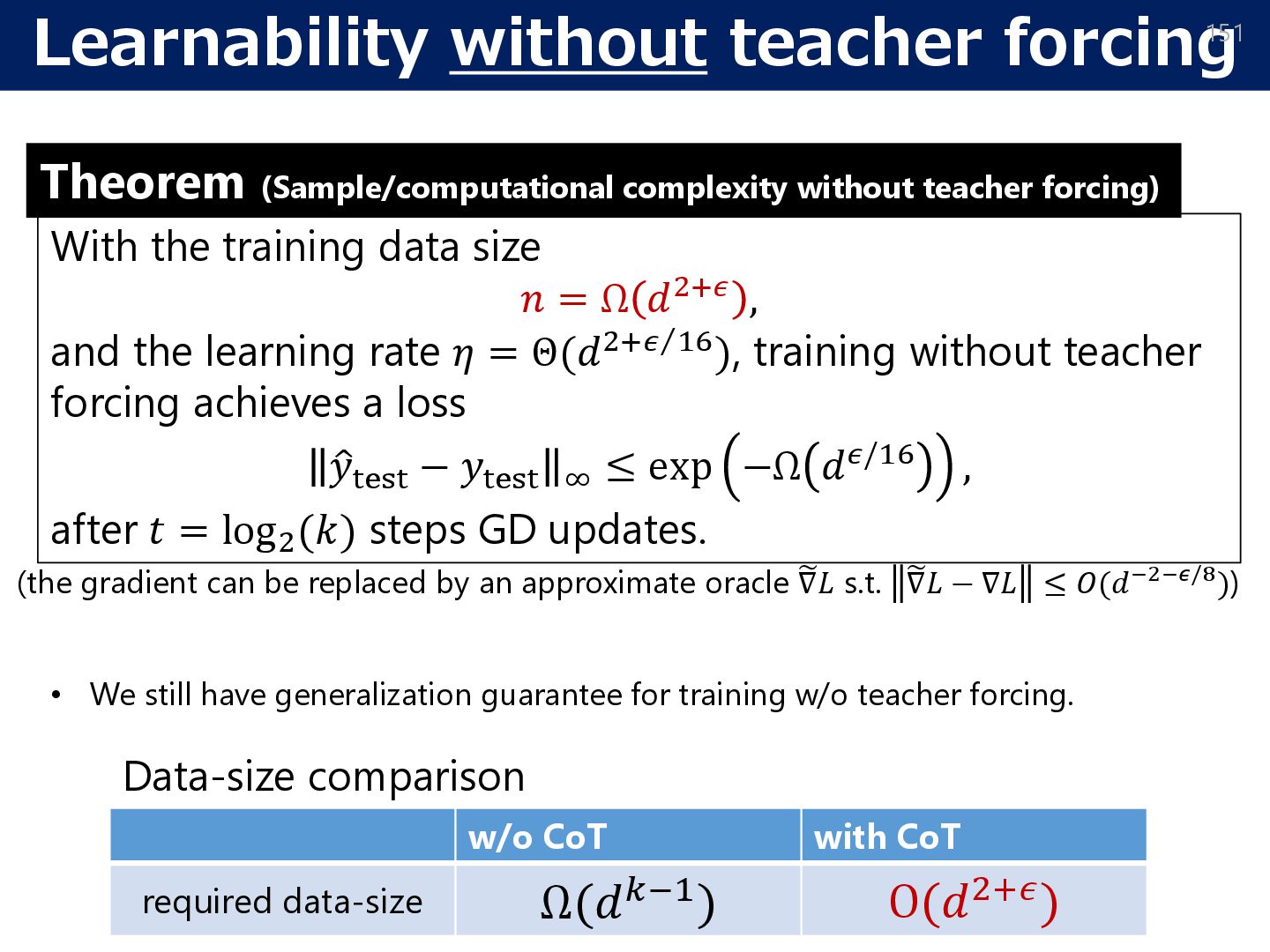
𝑛 = Ω 𝑑2+𝜖 , and the learning rate 𝜂 = Θ(𝑑2+ Τ 𝜖 16), training without teacher forcing achieves a loss ො 𝑦test − 𝑦test ∞ ≤ exp −Ω 𝑑𝜖/16 , after 𝑡 = log2 (𝑘) steps GD updates. Theorem (Sample/computational complexity without teacher forcing) w/o CoT with CoT required data-size Ω(𝑑𝑘−1) O(𝑑2+𝜖) Data-size comparison (the gradient can be replaced by an approximate oracle ෩ ∇𝐿 s.t. ෩ ∇𝐿 − ∇𝐿 ≤ 𝑂(𝑑−2−𝜖/8)) • We still have generalization guarantee for training w/o teacher forcing.
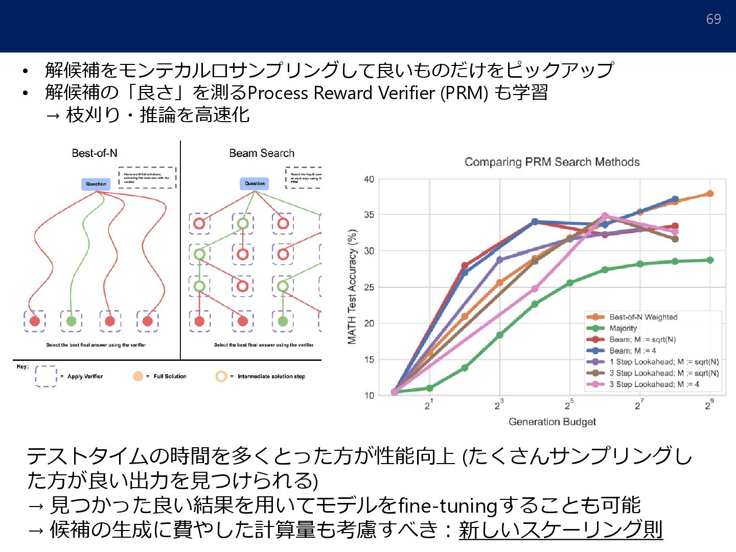
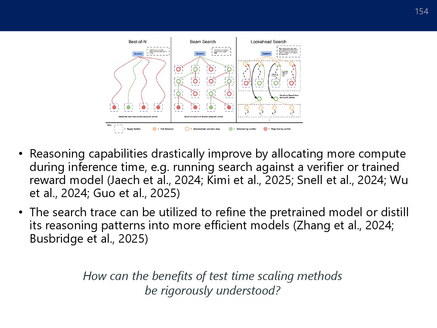
inference time, e.g. running search against a verifier or trained reward model (Jaech et al., 2024; Kimi et al., 2025; Snell et al., 2024; Wu et al., 2024; Guo et al., 2025) • The search trace can be utilized to refine the pretrained model or distill its reasoning patterns into more efficient models (Zhang et al., 2024; Busbridge et al., 2025) 154 How can the benefits of test time scaling methods be rigorously understood?
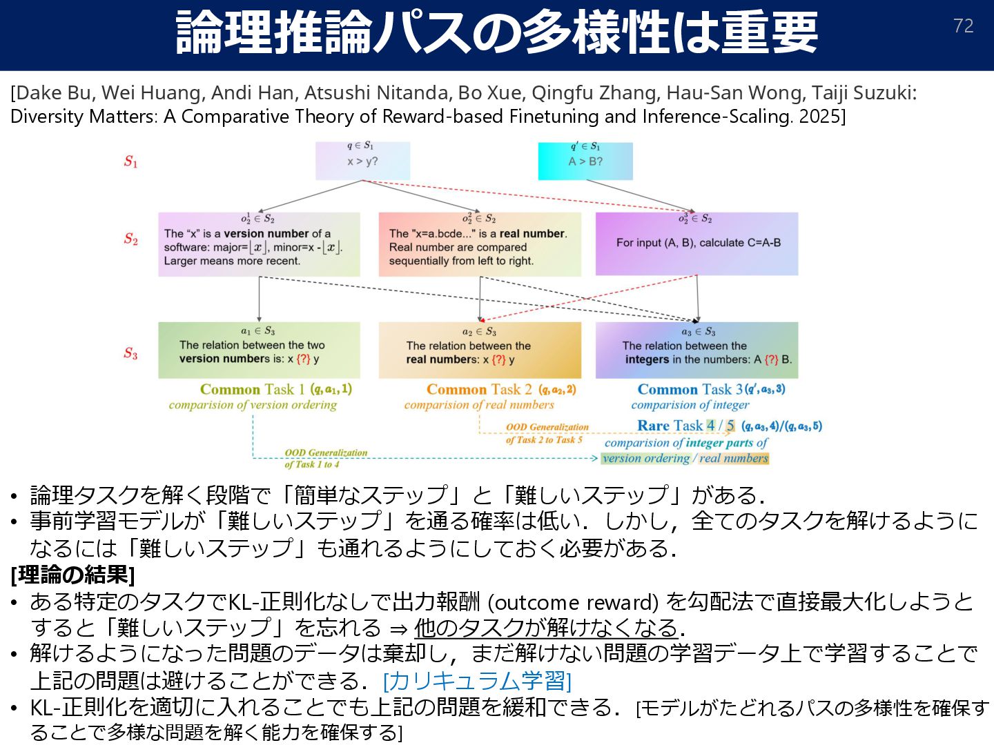
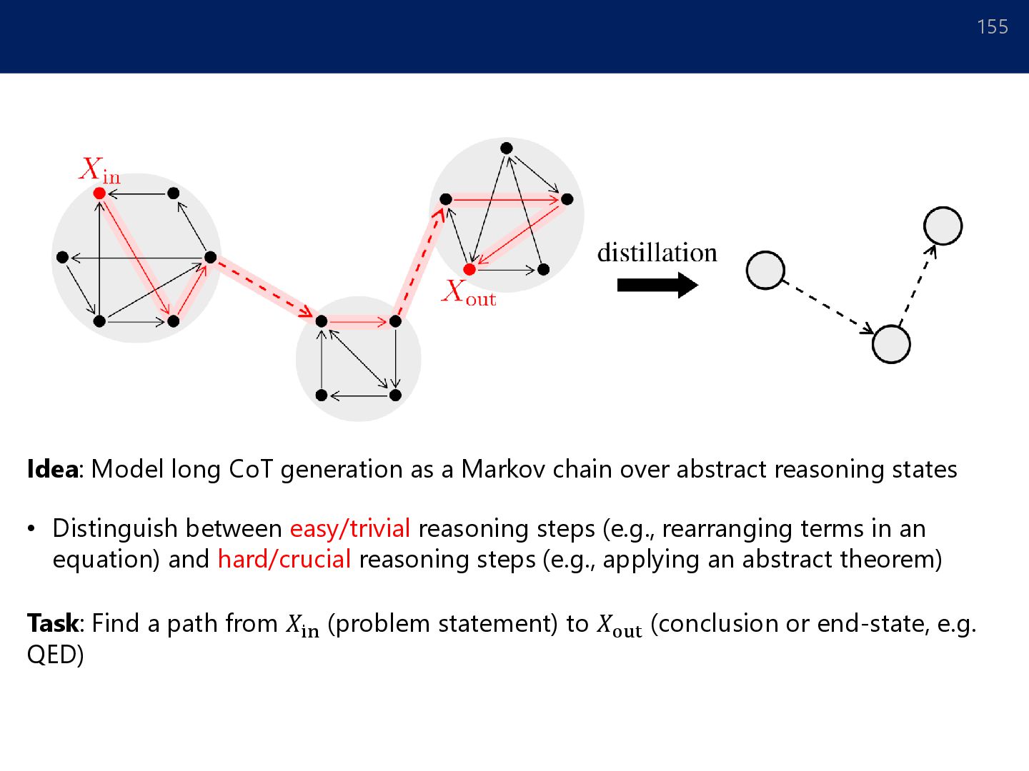
abstract reasoning states • Distinguish between easy/trivial reasoning steps (e.g., rearranging terms in an equation) and hard/crucial reasoning steps (e.g., applying an abstract theorem) Task: Find a path from 𝑋in (problem statement) to 𝑋out (conclusion or end-state, e.g. QED) 155
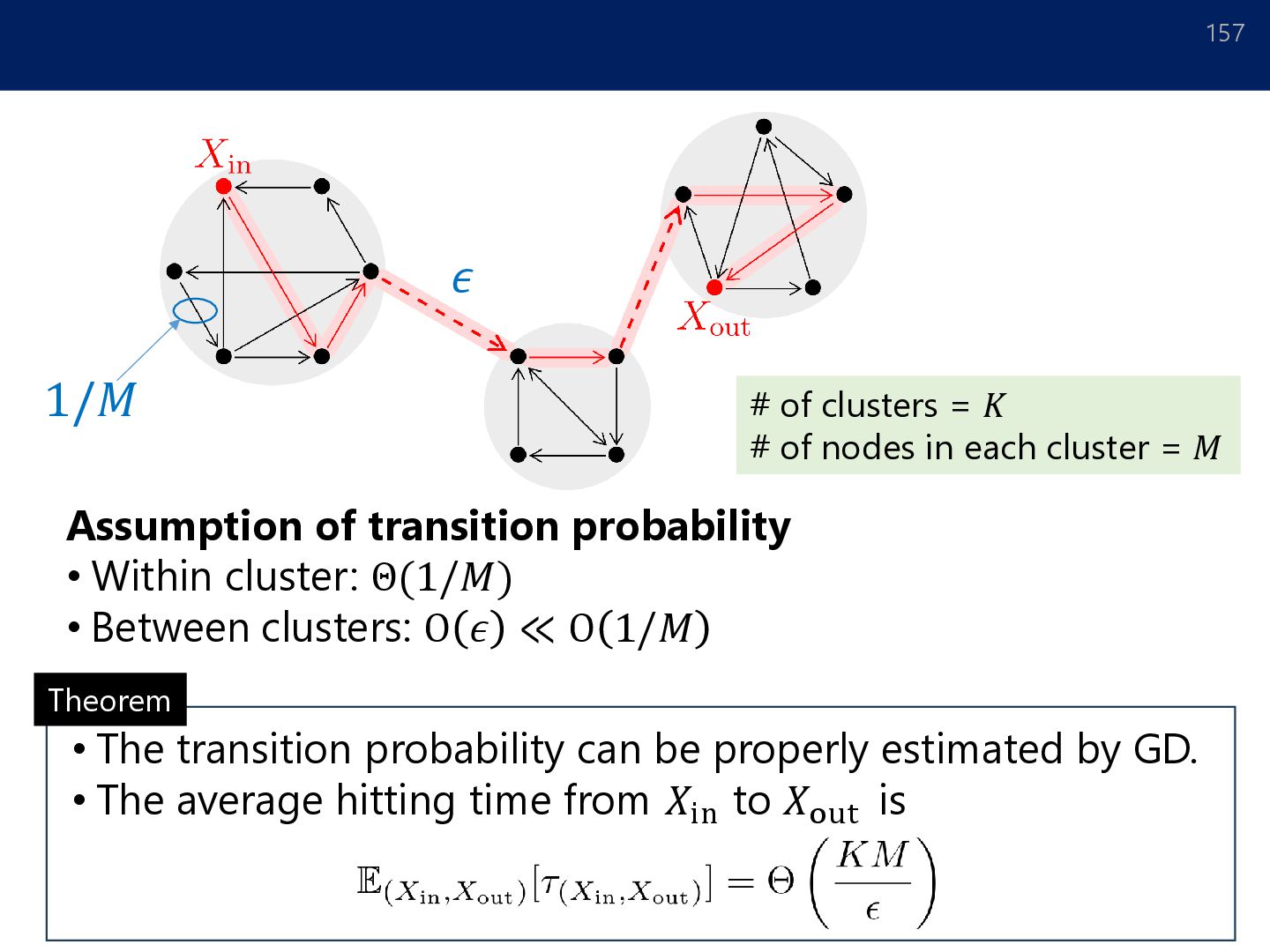
Between clusters: O 𝜖 ≪ O 1/𝑀 1/𝑀 𝜖 Theorem • The transition probability can be properly estimated by GD. • The average hitting time from 𝑋in to 𝑋out is # of clusters = 𝐾 # of nodes in each cluster = 𝑀
Between clusters: O 𝜖 ≪ O 1/𝑀 1/𝑀 𝜖 Theorem • The transition probability can be properly estimated by GD. • The average hitting time from 𝑋in to 𝑋out is # of clusters = 𝐾 # of nodes in each cluster = 𝑀
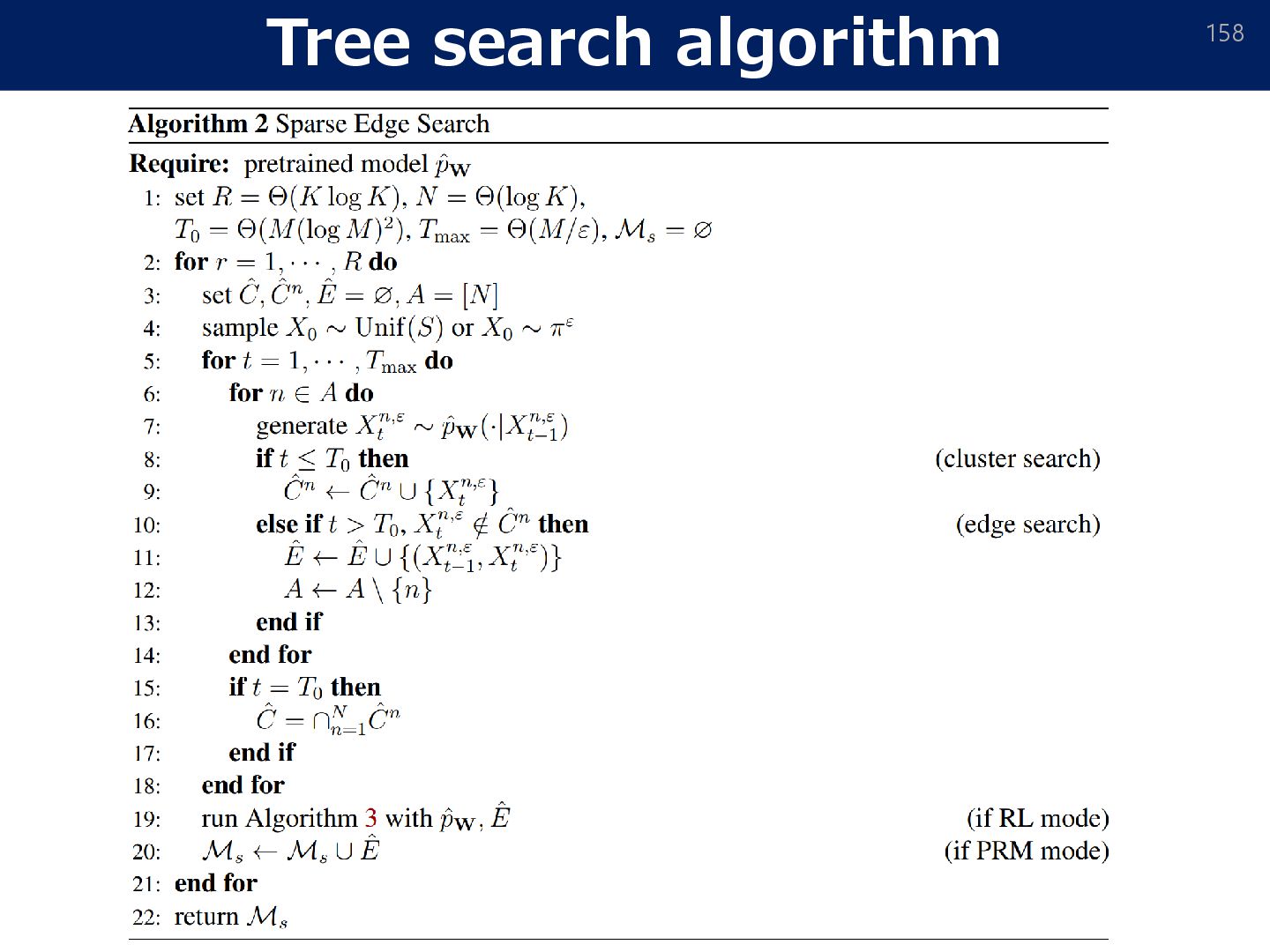
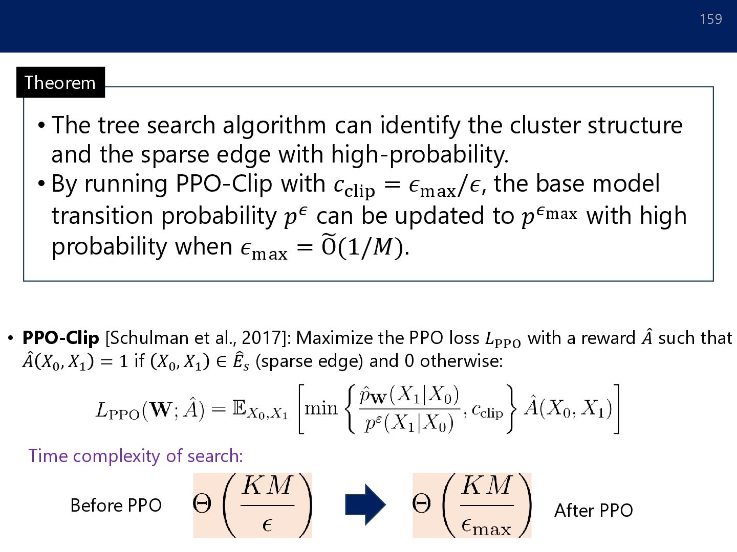
cluster structure and the sparse edge with high-probability. • By running PPO-Clip with 𝑐clip = 𝜖max /𝜖, the base model transition probability 𝑝𝜖 can be updated to 𝑝𝜖max with high probability when 𝜖max = ෩ O(1/𝑀). • PPO-Clip [Schulman et al., 2017]: Maximize the PPO loss 𝐿PPO with a reward መ 𝐴 such that መ 𝐴 𝑋0 , 𝑋1 = 1 if 𝑋0 , 𝑋1 ∈ 𝐸𝑠 (sparse edge) and 0 otherwise: Before PPO After PPO Time complexity of search:
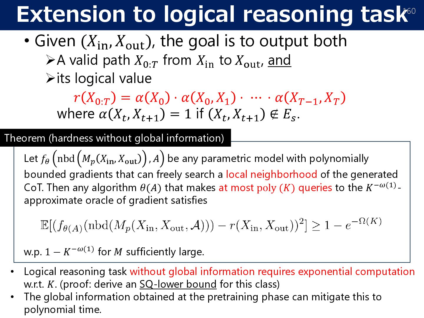
), the goal is to output both ➢A valid path 𝑋0:𝑇 from 𝑋in to 𝑋out , and ➢its logical value 𝑟 𝑋0:𝑇 = 𝛼 𝑋0 ⋅ 𝛼 𝑋0 , 𝑋1 ⋅ ⋯ ⋅ 𝛼 𝑋𝑇−1 , 𝑋𝑇 where 𝛼 𝑋𝑡 , 𝑋𝑡+1 = 1 if 𝑋𝑡 , 𝑋𝑡+1 ∉ 𝐸𝑠 . 160 Theorem (hardness without global information) Let 𝑓𝜃 nbd 𝑀𝑝 𝑋in , 𝑋out , 𝐴 be any parametric model with polynomially bounded gradients that can freely search a local neighborhood of the generated CoT. Then any algorithm 𝜃(𝐴) that makes at most poly (𝐾) queries to the 𝐾−𝜔(1)- approximate oracle of gradient satisfies w.p. 1 − 𝐾−𝜔(1) for 𝑀 sufficiently large. • Logical reasoning task without global information requires exponential computation w.r.t. 𝐾. (proof: derive an SQ-lower bound for this class) • The global information obtained at the pretraining phase can mitigate this to polynomial time.
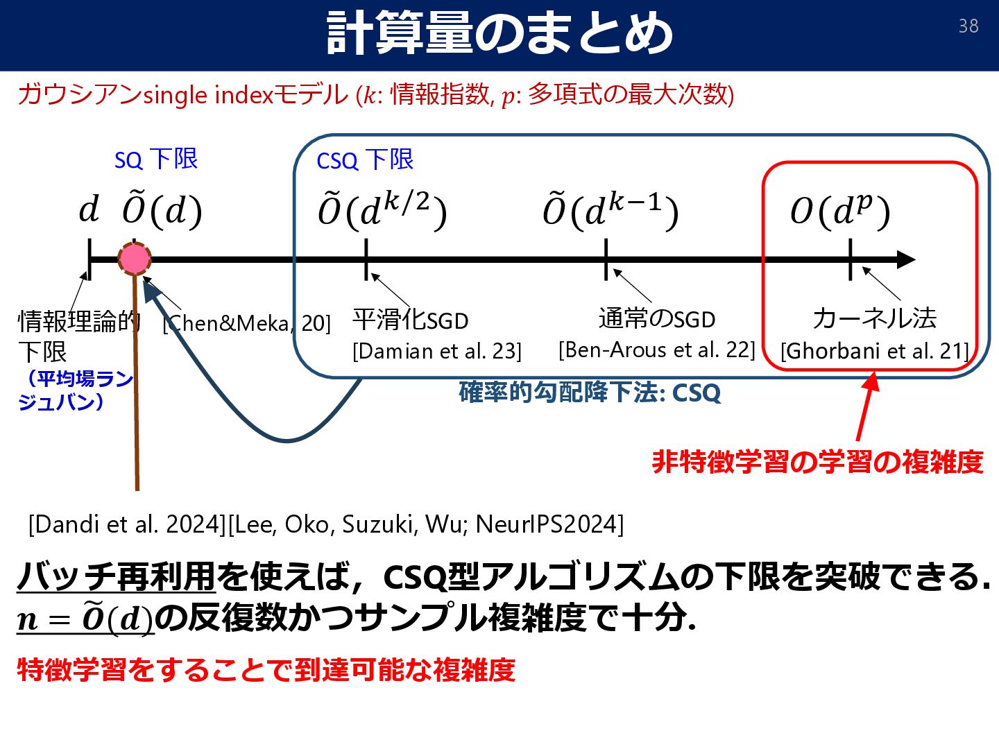
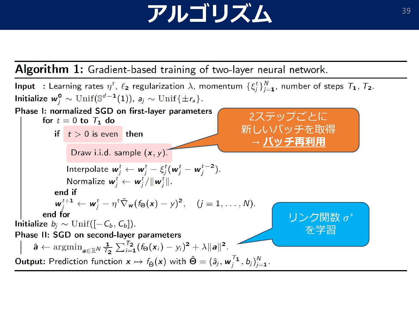
![バッチ再利用 • [Dandi et al. 2024] SGD + バッチ再利用 によってより高次の情報を取得](https://files.speakerdeck.com/presentations/d4f0f28b3c174275895e2d0e9f1e6ae0/slide_39.jpg)
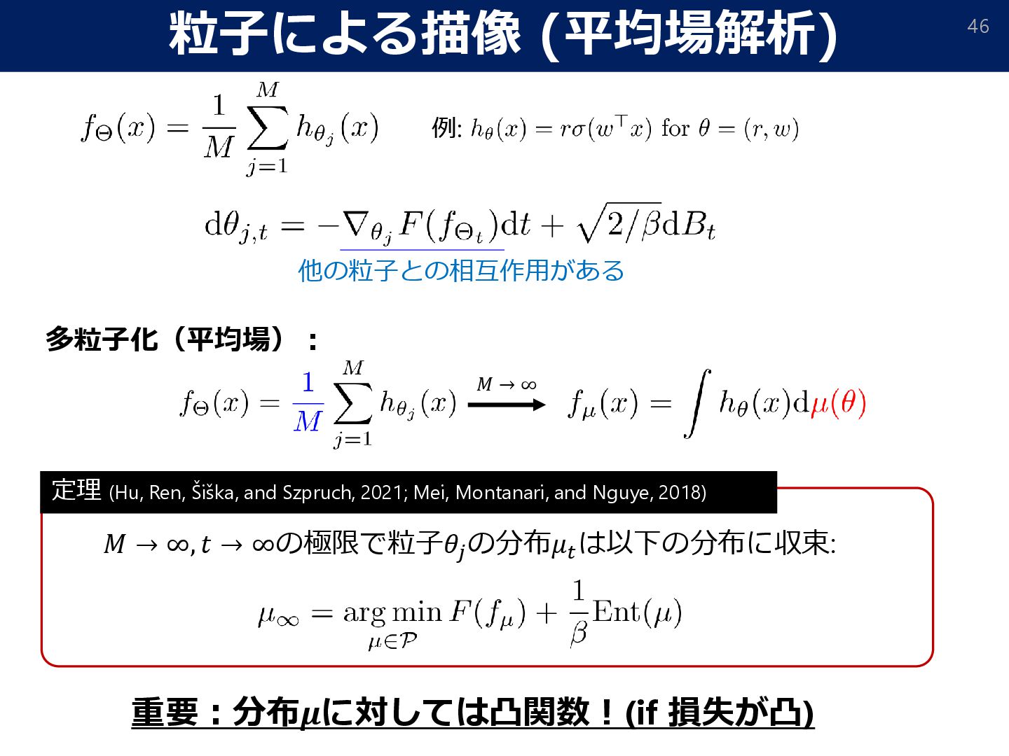
![粒子による分布の最適化 47 • 各ニューロンのパラメータを一つの粒子とみなす. • 各粒子が誤差を減らす方向に動くことで分布が最 適化される. 1つの粒子 [Nitanda&Suzuki, 2017][Chizat&Bach,](https://files.speakerdeck.com/presentations/d4f0f28b3c174275895e2d0e9f1e6ae0/slide_46.jpg)
![テスト時スケーリング 68 [ICLR2025, oral]](https://files.speakerdeck.com/presentations/d4f0f28b3c174275895e2d0e9f1e6ae0/slide_67.jpg)
![テスト時スケーリングの理論 (BoN) • BoN戦略から生成される出力の分布と元分布との差 [Beirami et al. 2025] 70 𝜋ref](https://files.speakerdeck.com/presentations/d4f0f28b3c174275895e2d0e9f1e6ae0/slide_69.jpg)
![Transformerの役割 • 事前学習 (pretraining): 特徴量 (表現) を学習 [𝑓∘] ➢Fourier, B-Spline](https://files.speakerdeck.com/presentations/d4f0f28b3c174275895e2d0e9f1e6ae0/slide_89.jpg)
![Transformerによる勾配法の実現 93 • Transformerは勾配法による文脈内学習を内部的に実装することができる. [勾配法の各更新が一層分に対応] • Transformerは交差検証法によるアルゴリズムの選択を内部的に実装できる. [Yu Bai, Fan](https://files.speakerdeck.com/presentations/d4f0f28b3c174275895e2d0e9f1e6ae0/slide_92.jpg)
![離散拡散モデルと言語生成 118 [Nie et al. Large Language Diffusion Models. arXiv:2502.09992]](https://files.speakerdeck.com/presentations/d4f0f28b3c174275895e2d0e9f1e6ae0/slide_117.jpg)
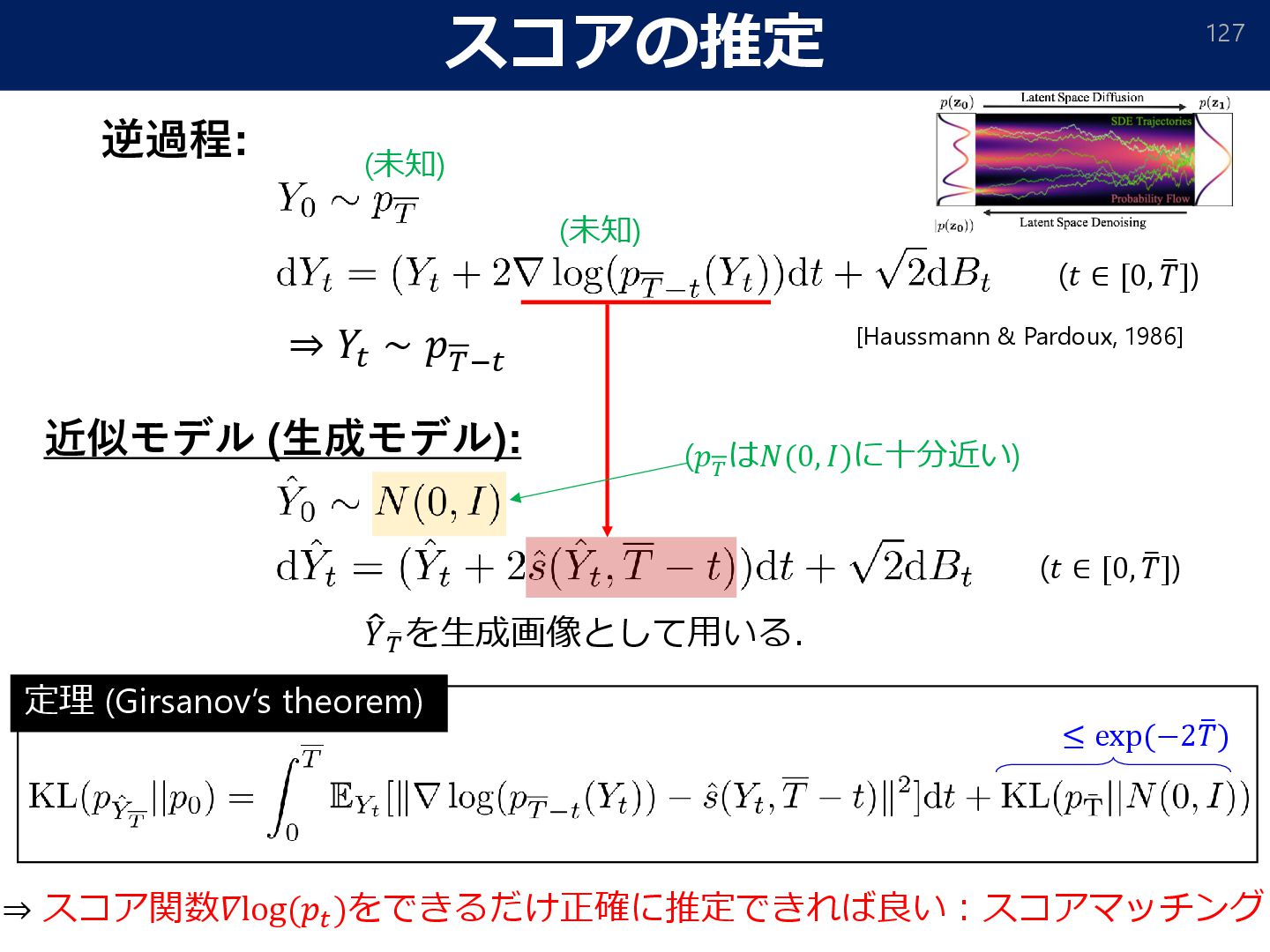
![逆過程 122 逆過程: [Haussmann & Pardoux, 1986] 事実:𝑌𝑡 の分布=𝑋ത 𝑇−𝑡](https://files.speakerdeck.com/presentations/d4f0f28b3c174275895e2d0e9f1e6ae0/slide_121.jpg)
![[参考] 線形推定量 147 例 • Kernel ridge estimator • Sieve](https://files.speakerdeck.com/presentations/d4f0f28b3c174275895e2d0e9f1e6ae0/slide_146.jpg)