Transport information Geometry: Current and Future II

The talk is presented at the conference: Further Developments of Information Geometry, the University of Tokyo, March 17-21, 2025.

Transcript

1. Transport Information Geometry: Current and Future Wuchen Li University of South Carolina This is mainly based on joint works with Jiaxi Zhao (NUS). Future Developments of Information Geometry, The University of Tokyo, March 20, 2025. Supported by the AFOSR YIP award.
2. Collaborators 2
3. Transport meets Information in Geometry 3
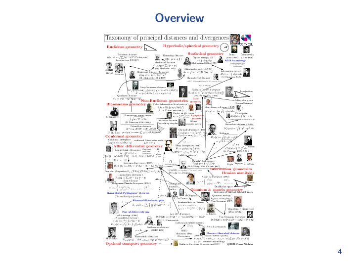
4. Overview Taxonomy of principal distances and divergences Euclidean geometry Information geometries Euclidean distance d2 (p, q) = i (pi − qi )2 (Pythagoras’ theorem circa 500 BC) Minkowski distance (Lk -norm) dk (p, q) = k i |pi − qi |k (H. Minkowski 1864-1909) Manhattan distance d1 (p, q) = i |pi − qi | (city block-taxi cab) Mahalanobis metric (1936) dΣ = (p − q)T Σ−1(p − q) Quadratic distance dQ = (p − q)T Q(p − q) Riemannian metric tensor gij dxi ds dxj ds ds (B. Riemann 1826-1866,) Physics entropy JK−1 −k p log pdµ (Boltzmann-Gibbs 1878) Information entropy H(p) = − p log pdµ (C. Shannon 1948) Fisher information (local entropy) I(θ) = E[ ∂ ∂θ ln p(X|θ) 2 ] (R. A. Fisher 1890-1962) Kullback-Leibler divergence KL(p||q) = p log p q dµ = Ep [log P Q ] (relative entropy, 1951) R´ enyi divergence (1961) Hα = 1 α(1−α) log fαdµ Rα (p|q) = 1 α(α−1) ln pαq1−αdµ (additive entropy) Tsallis entropy (1998) (Non-additive entropy) Tα (p) = 1 1−α ( pαdµ − 1) Tα (p||q) = 1 1−α (1 − pα qα−1 dµ) Bregman divergences (1967): BF (θ1 ||θ2 ) = F(θ1 ) − F(θ2 ) − (θ1 − θ2 )⊤∇F(θ2 ) Bregman-Csisz´ ar divergence (1991) Fα(x) = x − log x − 1 α = 0 x log x − x + 1 α = 1 1 α(1−α) (−xα + αx − α + 1) 0 < α < 1 Csisz´ ar’ f-divergence Df (p||q) = pf(q p )dµ (Ali& Silvey 1966, Csisz´ ar 1967) Amari α-divergence (1985) fα(x) = x log x α = 1 − log x α = −1 4 1−α2 (1 − x 1+α 2 ) −1 < α < 1 Quantum entropy S(ρ) = −kTr(ρ log ρ) (Von Neumann 1927) Kolmogorov K(p||q) = |q − p|dµ (Kolmogorov-Smirnoff max |p − q|) Hellinger H(p||q) = ( √ p − √ q)2 = 2(1 − √ fg Chernoff divergence (1952) Cα (p||q) = − ln pαq1−αdµ C(p, q) = maxα∈(0,1) Cα (p||q) χ2 test χ2(p||q) = (q−p)2 p dµ (K. Pearson, 1857-1936 ) Matsushita distance (1956) Mα (p, q) = α |q 1 α − p 1 α |dµ Bhattacharya distance (1967) d(p, q) = − log √ p √ qdµ Non-additive entropy cross-entropy conditional entropy mutual information (chain rules) Additive entropy Non-Euclidean geometries Statistical geometry Jeffrey divergence (Jensen-Shannon) H(p) = KL(p||u) Earth mover distance (EMD 1998) ×α(1 − α) α = −1 α = 0 Generalized Pythagoras’ theorem (Generalized projection) I-projection Quantum & matrix geometry Log Det divergence D(P||Q) =< P, Q−1 > − log det PQ−1 − dimP Von Neumann divergence D(P||Q) = Tr(P(log P − log Q) − P + Q) Itakura-Saito divergence IS(p|q) = i (pi qi − log pi qi − 1) (Burg entropy) Kullback-Leibler ∇∗ Hamming distance (|{i : pi ̸= qi }|) Neyman Dual div. (Legendre) DF ∗ (∇F(θ1 )||∇F(θ2 )) = DF (θ2 ||θ1 ) Generalized f-means duality... Dual div.∗-conjugate (f∗(y) = yf(1/y)) Df∗ (p||q) = Df (q||p) Burbea-Rao or Jensen (incl. Jensen-Shannon) JF (p; q) = f(p)+f(q) 2 − f p+q 2 Integral probability metrics IPMs Wasserstein distances Wα,ρ (p, q) = (infγ∈Γ(p,q) ρ(p, q)αdγ(x, y)) 1 α ρ = L1 L´ evy-Prokhorov distance LPρ (p, q) = infϵ>0 {p(A) ≤ q(Aϵ) + ϵ∀A ∈ B(X)} Aϵ = {y ∈ X, ∃x ∈ A : ρ(x, y) < ϵ} Finsler metric tensor gij = 1 2 ∂2 F 2(x,y) ∂yi∂yj Sharma-Mittal entropies hα,β (p) = 1 1−β pαdµ 1−β 1−α − 1 β = 1 β → α Fisher-Rao distance: ds2 = gij dθidθj = dθ⊤I(θ)dθ ρF R (p, q) = minγ 1 0 ˙ γ(t)I(θ) ˙ γ(t)dt Haussdorf set distance dH (X, Y ) = max{supx ρ(x, Y ), supy ρ(X, y)} Gromov-Haussdorf distance Sinkhorn divergence (h-regularized OT) (between compact metric spaces) dGH (X, Y ) = infϕX :X→Z,ϕY :Y →Z {ρZ H (ϕX (X), ϕY (Y ))} ϕX , ϕY : isometric embeddings MMD Maximum Mean Discrepancy Stein discrepancies ©2023 Frank Nielsen Optimal transport geometry Logarithmic divergence LG,α (θ1 : θ2 ) = 1 α log 1 + α∇G(θ2 )⊤(θ1 − θ2 ) +G(θ2 )−G(θ1 ) α → 0, F = −G Affine differential geometry Riemannian geometry Hyperbolic/spherical geometry Bolyai (1802-1860) Lobachevsky (1792-1856) Aitchison distance Probability simplex Hilbert log-ratio metric Quantum f-divergences (D´ enes Petz) Fr¨ obenius & Hilbert-Schmidt norm J. Jensen F. Itakura B. De Finetti G. Monge L. Kantorovich M. Nagumo Pearson K. Nomizu L. LeCam Vajda M. Fr´ echet J.M. Souriau J.L. Koszul Symplectic geometry Cone geometry E. Vinberg Bhat. Conformal geometry Conformal divergence Dρ (p : q) = ρ(p)D(p : q) conformal Riemannian metric gp hi = eϕg Dually flat space Constant sectional curvature Hessian manifolds H. Shima ∇ Lev M. Bregman C. R. Rao B. Riemann Euclid Pythagoras Pal & Wong 2016 4
5. Information matrix Information matrix (a.k.a Fisher information matrix, Fisher–Rao metric) plays important roles in estimation, information science, statistics and machine learning: ▶ Population Games via Replicator Dynamics (Shahshahani, Smith); ▶ Machine learning: Natural gradient (Amari); Adam (Kingma 2014); Stochastic relaxation (Malago) and many more in the book Information geometry (Ay et.al.). ▶ Statistics: Likelihood principle; Cramer-Rao bound, etc. 5
6. Learning Given a data measure ρdata (·) = 1 N N i=1 δXi (·) and a parameterized model ρ(·; θ). Machine learning problems often take the form min ρθ∈ρ(Θ) DKL (ρdata ||ρθ ). One typical choice of D is the Kullback–Leibler divergence (relative entropy) DKL (ρdata ||ρθ ) = Ω ρdata (x) log ρdata (x) ρ(x, θ) dx. 6
7. Natural gradient The natural gradient method is θk+1 = θk − hGF (θk)−1∇θ D(ρdata , ρθk ), where h > 0 is a stepsize and GF (θ) =EX∼ρθ (∇θ log ρ(X, θ))T (∇θ log ρ(X, θ)) is the Fisher information matrix. Why natural gradient and Fisher information matrix? ▶ Parameterization invariant; ▶ Pre-conditioners for KL divergence related learning problems; ▶ Online Cramer-Rao bound. 7
8. Optimal transport In recent years, optimal transport (a.k.a Earth mover’s distance, Monge-Kantorovich problem, Wasserstein metric) has witnessed a lot of applications: ▶ Population Games via Fokker-Planck Equations (Degond et. al. 2014, Li et.al. 2016); ▶ Machine learning: Wasserstein Training of Boltzmann Machines (Cuturi et.al. 2015); Learning from Wasserstein Loss (Frogner et.al. 2015); Wasserstein GAN (Bottou et.al. 2017); Wasserstein statistics, and many more in NIPS 2015–now. 8
9. Why optimal transport? Optimal transport provides a particular distance (W) among histograms, which relies on the distance on sample spaces (ground cost c). E.g. Denote X0 ∼ ρ0 = δx0 , X1 ∼ ρ1 = δx1 . Compare W(ρ0, ρ1) = inf π∈Π(ρ0,ρ1) E(X0,X1)∼π c(X0 , X1 ) = c(x0 , x1 ) Vs TV(ρ0, ρ1) = Ω |ρ0(x) − ρ1(x)|dx = 2 Vs KL(ρ0∥ρ1) = Ω ρ0(x) log ρ0(x) ρ1(x) dx = ∞. 9
10. Wasserstein Loss function Given a data distribution ρ0 and a probability model ρθ , consider min θ∈Θ W(ρ0, ρθ ). This is a double minimization problem, because W(ρ0, ρθ ) = min π∈Π(ρ0,ρθ) E(X0,X1)∼π c(X0 , X1 ). Many applications, such as Wasserstein GAN and Wasserstein loss are built on the above formulation. 10
11. Goals Main Question: Instead of looking at the Wasserstein distance, we propose the optimal transport induced information matrix in probability models, and study its properties in statistics and machine learning problems. Related studies ▶ Wasserstein covariance (Petersen, Muller ...) ▶ Wasserstein natural gradient (Li, Montufar, Chen, Lin, Abel, Liu ...) ▶ Wasserstein divergences (Wang, Pal, Guo, Li, Ay ...) ▶ Wasserstein statistics (Amari, Li, Matsuda, Zhao, Rubio ...) ▶ Wasserstein fluctuation and non-equilibrium thermodynamics (Ito, Kobayashi, Li, Liu, Gao ...) ▶ Wasserstein diffusions and Dean-Kawasaki dynamics (Renesse, Sturm, Li ...) ▶ ...... 11
12. Problem formulation ▶ Mapping formulation: Monge problem (1781): Monge-Amp´ ere equation ; ▶ Static formulation: Kantorovich problem (1940): Linear programming ; ▶ Dynamic formulation: Density optimal control (Nelson, Lafferty, Otto, Villani). In this talk, we will apply density optimal control into learning problems. 12
13. Density manifold Optimal transport has an optimal control reformulation by the dual of dual of linear programming: inf ρt 1 0 gW (∂t ρt , ∂t ρt )dt = 1 0 Ω (∇Φt , ∇Φt )ρt dxdt, under the dynamical constraint, i.e. continuity equation: ∂t ρt + ∇ · (ρt ∇Φt ) = 0, ρ0 = ρ0, ρ1 = ρ1. Here, (P(Ω), gW ) forms an infinite-dimensional Riemannian manifold1. 1John D. Lafferty: the density manifold and configuration space quantization, 1988. 13
14. Information matrix and Pull back 14
15. Statistical information matrix Definition (Statistical Information Matrix) Consider the density manifold (P(X), g) with a metric tensor g, and a smoothly parametrized statistical model pθ with parameter θ ∈ Θ ⊂ Rd. Then the pull-back G of g onto the parameter space Θ is given by G(θ) = ∇θ pθ , g(pθ )∇θ pθ . Denote G(θ) = (G(θ)ij )1≤i,j≤d , then G(θ)ij = X ∂ ∂θi p(x; θ) g(pθ ) ∂ ∂θj p (x; θ)dx. Here we name g the statistical metric, and call G the statistical information matrix. 15
16. Score Function Definition (Score Function) Denote Φi : X × Θ → R, i = 1, ..., n satisfying Φi (x; θ) = g(p) ∂ ∂θi p(x; θ) . They are the score functions associated with the statistical information matrix G and are equivalent classes in C(X)/R. The representatives in the equivalent classes are determined by the following normalization condition: Epθ Φi = 0, i = 1, ..., n. Then the statistical metric tensor satisfies G(θ)ij = X Φi (x; θ) g(pθ )−1Φj (x; θ)dx. 16
17. Example: Fisher-Rao metric ▶ The Fisher-Rao metric comes from Information Geometry. ▶ The inverse of the Fisher-Rao metric tensor is defined by GF (ρ)−1Φ = ρ Φ − Φρdx , Φ ∈ T∗ ρ P(Ω). ▶ For σ1 , σ2 ∈ Tρ P(Ω), the Fisher-Rao metric on the tangent space follows gF ρ (σ1 , σ2 ) = Φ1 Φ2 ρdx − Φ1 ρdx Φ2 ρdx , where Φi is the solution to σi = ρ Φi − Φi ρdx , i = 1, 2. 17
18. Example: Wasserstein metric ▶ The Wasserstein metric comes from Optimal Transport1. ▶ The inverse of the Wasserstein metric tensor is defined by GW (ρ)−1Φ = −∇ · (ρ∇Φ), Φ ∈ T∗ ρ P(Ω). ▶ The Wasserstein metric on the tangent space is given by gW ρ (σ1 , σ2 ) = ρ⟨∇Φ1 , ∇Φ2 ⟩dx, σ1 , σ2 ∈ Tρ P(Ω), where Φi is the solution to σi = −∇ · (ρ∇Φi ), i = 1, 2. 1C´ edric Villani. Topics in optimal transportation. American Mathematical Soc., 2003. 18
19. Wasserstein and Fisher score functions Proposition (Poisson equation) The Wasserstein score functions ΦW i (x; θ) satisfy the following Poisson equation ∇x log p(x; θ) · ∇x ΦW i (x; θ) + ∆x ΦW i (x; θ) = − ∂ ∂θi log p(x; θ). 19
20. WIM for independent models Proposition (Separability) If p(x; θ) is an independence model, i.e. p(x, θ) = Πn k=1 pk (xk ; θ), xk ∈ Xk , x = (x1 , · · · , xn ). Then there exists a set of one dimensional functions ΦW,k : Xk × Θk → R, such that ΦW (x; θ) = n k=1 ΦW,k(xk ; θ). In addition, the Wasserstein information matrix is separable: GW (θ) = n k=1 Gk W (θ), where Gk W (θ) = Epθ ∇xk ΦW,k(x; θ), ∇xk ΦW,k(x; θ) . 20
21. WIM in 1D Proposition (One dimensional sample space) If X ⊂ R1, the Wasserstein score functions satisfy ΦW i (x; θ) = − X∩(∞,x] 1 p(z; θ) ∂ ∂θi F(z; θ)dz, where F(x; θ) = X∩(∞,x] ρ(y; θ)dy is the cumulative distribution function. And the Wasserstein information matrix satisfies GW (θ)ij = Epθ ∂ ∂θi F(x; θ) ∂ ∂θj F(x; θ) p(x; θ)2 . 21
22. Remark ▶ The Wasserstein score function is the average of the cumulative Fisher score function. ▶ The Wasserstein information matrix is the covariance of the density average of the cumulative Fisher score function. 22
23. WIM in location-scale families Classical statistical models: ▶ Gaussian family: p(x; µ, σ) = 1 √ 2πσ e− 1 2σ2 (x−µ)2 , GW (µ, σ) = 1 0 0 1 . ▶ Laplacian family: p(x; m, λ) = λ 2 e−λ|x−m|, GW (m, λ) = 1 0 0 2 λ4 . 23
24. WIM in generative models Generative models: ▶ Continuous 1-d generative family: p(·; θ) = fθ∗ p0 (·) , p0 a given distribution, GW (θ) = |∇θ fθ (x)|2 p0 (x) dx, where the push-forward distribution is defined as A p0 dx = f−1 θ (A) fθ∗ p0 dx, 24
25. WIM in generative models Generative models: ▶ ReLU family: fθ (x) = σ (x − θ) = 0, x ≤ θ, x − θ, x > θ. GW (θ) = F0 (θ), F0 cumulative distribution function of p0 . ▶ Can we use this to analysis the dynamics systems appeared in machine learning? 25
26. Classical (Fisher) statistics & Wasserstein statistics We develop a parallel Wasserstein statistics following the classical statistics approach ▶ Covariance inner product −→ Wasserstein covariance ▶ Cramer-Rao bound cotangent space −→ Wasserstein-Cramer-Rao bound ▶ Natural gradient efficiency separability −→ Wasserstein Natural gradient efficiency 26
27. Wasserstein covariance Definition (Wasserstein covariance) Given a statistical model Θ, denote the Wasserstein covariance as follows: CovW θ [T1 , T2 ] = Epθ ∇x T1 (x), ∇x T2 (x)T , where T1 , T2 are random variables as functions of x and the expectation is taken w.r.t. x ∼ pθ . Denote the Wasserstein variance: VarW θ [T] = Epθ ∇x T(x), ∇x T(x)T . Problem How does the Wasserstein covariance describe the variance of an estimator? 27
28. Wasserstein-Cramer-Rao bound Theorem (Wasserstein-Cramer-Rao inequalities) Given any set of statistics T = (T1 , ..., Tn ) : X → Rn, where n is the number of the statistics, define two matrices CovW θ [T(x)], ∇θEpθ [T(x)]T as below: CovW θ [T(x)]ij = CovW θ [Ti , Tj ], ∇θEpθ [T(x)]T ij = ∂ ∂θj Epθ [Ti (x)], then CovW θ [T(x)] ⪰ ∇θEpθ [T(x)]T GW (θ)−1∇θEpθ [T(x)]. 28
29. Cramer-Rao bound: Classical and Wasserstein ▶ Gaussian: GW (µ, σ) = 1 0 0 1 , GF (µ, σ) = 1 σ2 0 0 2 σ2 . ▶ Laplacian: GW (m, λ) = 1 1 λ2 1 λ2 2 λ4 , GF not well-defined. ▶ Comparison: GW is well-defined for wider range of families. ▶ Tighter bound on the variance of an estimator 29
30. Functional inequalities Wasserstein geometry is related to functional inequalities. Study both the global version (density manifold) and local version (statistical manifold). ▶ Dissipation of entropy & Fisher information functional d dt DKL (p∥q) = − X ∥∇x log p(x) q(x) ∥2p(x)dx = − I(p∥q) (global version) d dt DKL (pθ ∥pθ∗ ) = −∇θ DT KL G−1 W ∇θ DKL =: − ˜ I(θ∥θ∗) (local version) ▶ Log-Sobolev inequality DKL (p∥q) ≤ 1 2α I(p∥q), p ∈ P(X) (global version) DKL (pθ ∥pθ∗ ) ≤ 1 2α I(θ∥θ∗ ), θ ∈ Θ (local version) 30
31. Functional inequalities Theorem (Ricci-Information-Wasserstein-condition) The information matrix criterion for log-Sobolev inequality can be written as: GF (θ) + ∇2 θ pθ log pθ pθ∗ − ΓW · ∇θ DKL (pθ ∥pθ∗ ) ≥ 2αGW (θ), where ΓW is the Christoffel symbol in Wasserstein statistical model Θ, while for Poincare inequality can be written as: GF (θ) + ∇2 θ pθ log pθ pθ∗ ≥ 2αGW (θ). 31
32. Wasserstein natural gradient Definition (Wasserstein natural gradient) Given a statistical model Θ and a loss function l: Θ → R. The Wasserstein natural gradient is defined by ∇W θ l(θ) = G−1 W (θ)∇l(θ), where ∇l(θ) is the Euclidean gradient operator of loss function. 32
33. Online natural gradient algorithm We sample from the unknown distribution once in each step, and use sample xt to get new estimator θt+1 θt+1 = θt − 1 t ∇W θ l(xt , θt ). In order to analysis the convergence of this online algorithm, we define the Wasserstein covariance matrix Vt to be Vt = Epθ∗ ∇(θt − θ∗ ) · ∇(θt − θ∗ )T , where θ∗ is the optimal value. Definition (Natural gradient efficiency) The Wasserstein natural gradient is asymptotic efficient if Vt = 1 t G−1 W (θ∗ ) + O( 1 t2 ). 33
34. Theorem on updation of the covariance Theorem (Variance updating equation of the Wasserstein Natural Gradient) For any function l(x, θ) that satisfies the condition Epθ l(x, θ) = 0, consider here the asymptotic behavior of the Wasserstein dynamics θt+1 = θt − 1 t G−1 W (θt )l(xt , θt ). That is, assume priorly Epθ∗ (θt − θ∗ )2 , Epθ∗ |∇x (θt − θ∗ )|2 = o(1), ∀t. Then, the Wasserstein covariance matrix Vt updates according to the following equation: Vt+1 = Vt + 1 t2 G−1 W (θ∗ )Epθ∗ ∇x (l(xt , θ∗ )) · ∇x l(xt , θ∗ )T G−1 W (θ∗ ) − 2Vt t Epθ∗ [∇θ l(xt , θ∗ )] G−1 W (θ∗ ) + o( Vt t ) + o 1 t2 . 34
35. Natural gradient efficiency Theorem (Wasserstein Natural Gradient Efficiency) For the dynamics θt+1 = θt − 1 t G−1 W (θt )l(xt , θt ), the Wasserstein covariance updates according to Vt+1 =Vt + 1 t2 G−1 W (θ∗ ) − 2 t Vt + o 1 t2 + o( Vt t ). Then, the online Wasserstein natural gradient algorithm is Wasserstein efficient, that is: Vt = 1 t G−1 W (θ∗ ) + O 1 t2 . 35
36. Poincare Efficiency Corollary (Poincare Efficiency) For the dynamics θt+1 = θt − 1 t ∇W θ l(xt , θt ), the Wasserstein covariance updates according to Vt+1 = Vt + 1 t2 G−1 W (θ∗ )Epθ∗ ∇x (∇θ l(xt , θ∗ )) · ∇x ∇θ l(xt , θ∗ )T G−1 W (θ∗ ) − 2 t Vt GF (θ∗ )G−1 W (θ∗ ) + O 1 t3 + o Vt t . Now suppose that α = sup{a|GF ⪰ aGW }. Then the dynamics is characterized by the following formula Vt =      O t−2α , 2α ≤ 1, 1 t 2GF G−1 W − I −1 G−1 W (θ∗ )IG−1 W (θ∗ ) + O 1 t2 , 2α > 1, where I = Epθ∗ ∇x (∇θ l(xt , θ∗ )) · ∇x ∇θ l(xt , θ∗ )T . 36
37. I: WIM for one-dimensional Gaussian mixture models 37
38. Gaussian mixture model (GMM) Gaussian mixture models (GMM) are widely used in statistical inference (statistical models) and scientific computation. A simple review of GMM: ρ : Θ → P (R) , Θ ⊂ RN−1, θ → ρθ = N−1 i=1 θi (ρi+1 − ρi ) + ρ1 = N i=1 pi ρi , 1 = θ0 > θ1 > · · · > θN−1 > θN = 0, ρi ∼ N µi , σ2 , µ1 < µ2 < · · · < µN−1 < µN , This work is based on the consideration of GMM. 2Li, Wuchen, and Jiaxi Zhao. ”Scaling limits of the Wasserstein information matrix on Gaussian mixture models.” arXiv preprint arXiv:2309.12997 (2023). 38
39. Our approach We characterize the TIG of GMMs in the asymptotic regime. Rescale GMMs to approximate discrete spaces. As the variance of Gaussian tends to 0, distributions weakly converge to a Dirac measure: lim σ→0 GW (θ; σ) K (σ) = G W (θ) . 39
40. Scaling approximation Fisher-Rao metric Theorem (Scaling Fisher-Rao metric) For a 1-d homogeneous GMM, the above scaling limit of Fisher information matrices is given by G F (θ) = lim σ→0 GF (θ; σ) =          1 p1 + 1 p2 − 1 p2 0 · · · 0 0 − 1 p2 1 p2 + 1 p3 − 1 p3 · · · 0 0 0 − 1 p3 1 p3 + 1 p4 · · · 0 0 . . . . . . . . . ... . . . . . . 0 0 0 · · · − 1 pN−1 1 pN−1 + 1 pN          . 40
41. Wasserstein pull-back metric on GMM Example Explicit formula for Wasserstein metric in one-dimensional sample space reads GW (θ)ij = Eρθ ∂ ∂θi F(x; θ) ∂ ∂θj F(x; θ) ρ(x; θ)2 , where F(x; θ) is the cumulative distribution function of the density function ρ(x; θ). In case of GMM, it is given by GW (θ)ij = Eρθ (Fi+1 (x; θ) − Fi (x; θ)) (Fj+1 (x; θ) − Fj (x; θ)) ρ(x; θ)2 , where Fi (x; θ) is the cumulative distribution function of the density function ρi (x; θ). 41
42. Scaling approximation Wasserstein metric Theorem (Scaling Wasserstein metric) For a 1-d homogeneous GMM with difference between adjacent components given by d, a scaling limit of Wasserstein information matrices is given by G W (θ) = lim σ→0 GW (θ; σ) K (σ) =           1 √ p1p2 0 0 · · · 0 0 0 1 √ p2p3 0 · · · 0 0 0 0 1 √ p3p4 · · · 0 0 . . . . . . . . . ... . . . . . . 0 0 0 · · · 0 1 √ pN−1pN           The scaling factor appearing above is given by K (σ) = √ 2π3 σ3 d e1 2 ( d 2σ )2 . 42
43. Scaling approximation Wasserstein metric Sketch of proof: (GW (θ)) i−1,i−1 = (Fi − Fi−1 )2 ρθ dx ∆1 =⇒ µi µi−1 1 pi−1 ρi−1 + pi ρi dx ∆2 =⇒ Laplacian asymptotics. 43
44. Inhomogeneous GMM What if the gap between adjacent components are not the same? µi+1 − µi ̸= µj+1 − µj ▶ Homogeneous lattice ⇐⇒ GMM with same variances for components. ▶ Inhomogeneous lattice ⇐⇒ GMM with different variances for components. Theorem (informal) For a 1-d inhomogeneous GMM with difference between adjacent components given by µi+1 − µi = di , choose the variances of components as σi = si σ such that the condition below is satisfied d1 s1 + s2 = d2 s2 + s3 = · · · = dN−1 sN−1 + sN = d. (1) A scaling limit of Wasserstein information matrices is again diagonal. 44
45. Extended GMM Now, we discuss an extended GMM, which is able to be tackled in our framework. Recall GMMs as: ρθ = N−1 i=1 θi (ρi+1 − ρi ) + ρ1 , θi−1 ≥ θi ≥ 0, ∀i = 2, ..., N, ρi ∼ N (µi , σ) , ∀i = 1, ..., N. In ordinary GMMs, the µi s are constants while only θi s are parameters. In extended GMMs, both these two sets are parameters, namely, the means of each components can vary. 45
46. Extended GMMs and Wasserstein information geometry Theorem (Wasserstein information geometry of extended GMMs) For the extended GMM, we have the following relationship between the Wasserstein information matrix(WIM) of the set of tangent vectors ∂ ∂µi s and Fisher information matrix(FIM) of the set of tangent vectors ∂ ∂θi s GF = ΣGW ΣT , where (GF ) ij = gF ∂ ∂θi , ∂ ∂θj , (GW ) ij = gW ∂ ∂µi , ∂ ∂µj and the matrix Σ ∈ RN−1,N appears above is given by Σ =          − 1 p1 1 p2 0 · · · 0 0 0 − 1 p2 1 p2 · · · 0 0 . . . . . . ... · · · · · · · · · 0 0 · · · − 1 pN−2 1 pN−1 0 0 0 0 · · · − 1 pN−1 1 pN          . 46
47. II: WIM for one-dimensional generative models 47
48. Scientific computing applications Can we apply this framework to the scientific computing applications and propose novel numerical methods?3 3Zuo, Xinzhe, et al. ”Numerical Analysis on Neural Network Projected Schemes for Approximating One Dimensional Wasserstein Gradient Flows.” arXiv preprint arXiv:2402.16821 (2024). 48
49. Generative probability models Consider a class of invertible push-forward maps {fθ }θ∈Θ indexed by parameter θ ∈ Θ ⊂ RD fθ : Rd → Rd. We obtain a family of parametric distributions PΘ = ρθ = fθ# p | θ ∈ Θ ⊂ (P, gW ). Combine the generative models with TIG to design numerical methods. 49
50. Wasserstein gradient flow (Lagrangian formulation) Define the pushforward of pr by T as p(x) = T# pr (x) ≜ pr |det(Dz T)| ◦ T−1(x). Then, F(p) can be viewed as a functional of T, F#(T) ≜ F(T# pr ). Wasserstein gradient flow of F#(T) yields the dynamic: ∂t T(t, ·) = −gradW F#(T(t, ·)) ≜ − 1 pr (·) δF#(T(t, ·)) δT (·). (2) 50
51. Neural network functions Consider a mapping function f : Z × Θ → Ω, where Z ⊂ Rl is the latent space, Ω ⊂ Rd is the sample space and Θ ⊂ RD is the parameter space. f(θ, z) = 1 N N i=1 ai σ z − bi , where θ = (ai , bi ) ∈ RD, D = (l + 1)N. Here N is the number of hidden units (neurons). ai ∈ R is the weight of unit i. bi ∈ Rl is an offset (location variable). σ: R → R is an activation function, which satisfies σ(0) = 0, 1 ∈ ∂σ(0). z σ x Example (ReLU) Denote σ(x) = max{x, 0}. Suppose N = d = 1, then f(θ, z) = θ max{z, 0}, θ ∈ R+ . 51
52. Models Definition (Neural mapping models) Let us define a fixed input reference probability density pr ∈ P(Z) = p(z) ∈ C∞(Z): Z pr (z)dz = 1, p(z) ≥ 0 . Denote a probability density generated by a neural network mapping function by the pushforward operator: p = fθ# pr ∈ P(Ω), In other words, p satisfies the following Monge-Amp` ere equation by p(f(θ, z))det(Dz f(θ, z)) = pr (z) , where Dz f(θ, z) is the Jacobian of the mapping function f(θ, z) w.r.t. variable z. 52
53. Wasserstein information distance Definition (Wasserstein mapping distance) Define a distance function DistW : Θ × Θ → R as DistW (fθ0 # pr , fθ1 # pr )2 = Z ∥f(θ0, z) − f(θ1, z)∥2pr (z)dz = d m=1 Ez∼pr ∥fm (θ0, z) − fm (θ1, z)∥2 , where θ0, θ1 ∈ Θ are two sets of neural network parameters and ∥ · ∥ is the Euclidean norm in Rd. 53
54. Generalized Wasserstein information matrix Consider the Taylor expansion of the distance function. Let ∆θ ∈ RD, DistW (fθ+∆θ# pr , fθ# pr )2 = d m=1 Ez∼pr ∥fm (θ + ∆θ, z) − fm (θ, z)∥2 = d m=1 D i=1 D j=1 Ez∼pr ∂θi fm (θ, z)∂θj fm (θ, z) ∆θi ∆θj + o(∥∆θ∥2) =∆θT GW (θ)∆θ + o(∥∆θ∥2). Here GW is a Gram-type matrix function: GW (θ) = Z ∇θ f(θ, z)∇θ f(θ, z)T pr (z)dz. 54
55. Wasserstein natural gradient flows in generative models Consider an energy functional F : P(Ω) → R. Then the gradient flow of function F(θ) = F(fθ# pr ) in (Θ, GW ) is given by dθ dt = −gradW F(θ) = −GW (θ)−1∇θ F(θ). In particular, dθi dt = − D j=1 d m=1 Ez∼pr ∇θ f(θ, z)∇θ f(θ, z)T −1 ij · E˜ z∼pr ∇xm δ δp F(p)(f(θ, ˜ z)) · ∂θj fm (θ, ˜ z) , where δ δp(x) is the L2–first variation w.r.t. variable p(x), x = f(θ, z). 55
56. Example I: Linear energy For the potential energy: F(p) = Ω V (x)p(x)dx. The Wasserstein gradient flow satisfies ∂t p(t, x) = ∇x · p(t, x)∇x V (x) . The Wasserstein natural gradient flow satisfies dθi dt = − D j=1 Ez∼pr ∇θ f(θ, z)∇θ f(θ, z)T −1 ij · E˜ z∼pr ∇x V (f(θ, ˜ z)) · ∂θj f(θ, ˜ z) . 56
57. Example II: Interaction energy For the interaction energy: F(p) = 1 2 Ω Ω W(x, y)p(x)p(y)dxdy. The Wasserstein gradient flow satisfies ∂t p(t, x) = ∇x · p(t, x) Ω ∇x W(x, y)p(t, y)dy . The neural projected dynamic satisfies dθi dt = − D j=1 Ez∼pr ∇θ f(θ, z)∇θ f(θ, z)T −1 ij · E(z1,z2)∼pr×pr ∇x1 W(f(θ, z1 ), f(θ, z2 )) · ∂θj f(θ, z1 ) . 57
58. Example III: Internal energy For the internal energy: F(p) = Ω U(p(x))dx. The Wasserstein gradient flow satisfies ∂t p(t, x) = ∇x · p(t, x)∇x U′(p(t, x)) . The neural projected dynamic satisfies dθi dt = − D j=1 Ez∼pr ∇θ f(θ, z)∇θ f(θ, z)T −1 ij · Ez∼pr − tr Dz f(θ, z)−1 : ∂θj Dz f(θ, z) ˆ U′( pr (z) det(Dz f(θ, z)) ) pr (z) det(Dz f(θ, z)) , where ˆ U(z) = 1 z U(z). 58
59. Analytic formula for WIM For a special case of 2-layer ReLU neural network with f(θ, z) = 1 N N i=1 ai σ(z − bi ), where only bi , i = 1, · · · , N can vary, we prove that the inverse matrix has the closed form 1 N2 G−1 W (b) ij =              − 1 ai ai−1 1 F0 (bi ) − F0 (bi−1 ) , j = i − 1, − 1 ai ai+1 1 F0 (bi+1 ) − F0 (bi ) , j = i + 1, 0, o.w. where F0 (·) is the cumulative distribution function of pr (·), i.e., F0 (x) = x −∞ pr (y)dy. 59
60. Consistency via analytic formula Consider ∂t p(t, x) = ∇ · (p(t, x)∇V (x)). Its neural projected dynamics satisfies dθ dt = −G−1 W (θ) · E˜ z∼pr ∇θ V (f(θ, ˜ z)) . The above ODE has a closed-form update: ˙ bi = N ai Ez∼pr [V ′(f(b, z))1[bi,bi+1] ] F0 (bi+1 ) − F0 (bi ) − Ez∼pr [V ′(f(b, z))1[bi−1,bi] ] F0 (bi ) − F0 (bi−1 ) , We need to show that the numerical scheme in the third line is consistent w.r.t. the original PDE in the first line. Proposition (Consistency of the projected potential flow) Assume potential functional satisfies ∥V ′′∥ ∞ < ∞. The spatial discretization is of first-order accuracy both in the mapping and the density coordinates. 60
61. Well-posedness for projected heat flow The project gradient flow of the entropy functional, i.e. the heat flow is given by ˙ bi = 1 F0 (bi ) − F0 (bi−1 )    log i−1 j=1 aj i j=1 aj pr (bi ) a2 i − log i−2 j=1 aj i−1 j=1 aj pr (bi−1 ) ai ai−1    + 1 F0 (bi+1 ) − F0 (bi )    log i−1 j=1 aj i j=1 aj pr (bi ) a2 i − log i j=1 aj i+1 j=1 aj pr (bi+1 ) ai ai+1    . This is a nonlinear ODE although the original heat equation is a linear PDE, but we can prove the well-posedness of the projected dynamics by analyzing the behavior of the adjacent modes. Proposition The neural projected dynamics of the heat flow is well-posed, e.g. the solution extends to arbitrary time. 61
62. Consistency analysis for general cases Previous analysis is based on either the analytic formula or specific gradient flow equation, we can also establish the consistency by viewing our method as a projection-based reduced order model, i.e. the projected gradient is chosen to minimize the Wasserstein inner product as illustrated below ∇θ H(θ) = argminv∈TθΘ (∇θ H(θ)(x) − v(x))2fθ# pr (x)dx, The L2-error between the projected gradient and original gradient is bounded by v(x) − ∇θ H(θ) 2 L2(fθ#pr) = 1 4 N j=1 aj N 2 ∥v′′∥ ∞ O(∆b4). Proposition The numerical scheme based on ReLU network mapping is consistent with order 2 using both a, b parameters and of order 1 with either a or b parameters. 62
63. Neural network structure We focus on the two-layer neural network with ReLU as activation functions. f(θ, z) = N i=1 ai · σ(z − bi ) + 2N i=N+1 ai · σ(bi − z) . θ ∈ R4N represents the collection of weights {ai }2N i=1 and bias {bi }2N i=1 . At initialization, we set ai = 1/N for i ∈ {1, . . . , N} and ai = −1/N for i ∈ {N + 1, . . . , 2N}. To choose the bi ’s, we first set b = linspace(−B, B, N) for some positive constant B (e.g. B = 4 or B = 10). We then set bi = b[i] for i = 1, . . . , N and bj = b[j − N] + ε for j = N + 1, . . . , 2N. Here ε = 5 × 10−6 is a small offset. Our initialization is chosen such that f(θ, ·) approximates the identity map at initialization. 63
64. Porous medium equation Consider the functional U(p(x)) = 1 m−1 p(x)m, m = 2. This choice of U yields the porous medium equation ∂t p(t, x) = ∆p(t, x)m . (3) 0.6 0.8 1.0 1.2 1.4 3.75 3.70 3.65 3.60 3.55 3.50 3.45 (a) Error 3 2 1 0 1 2 3 4 3 2 1 0 1 2 3 4 analytic computed (b) Mapping comparison 2 1 0 1 2 0.0 0.2 t=0.000 2 1 0 1 2 0.0 0.2 t=0.200 2 0 2 0.0 0.2 t=0.400 2 0 2 0.0 0.2 t=0.600 2 0 2 0.0 0.2 t=0.800 2 0 2 0.0 0.2 t=1.000 (c) Density evolution Figure: Left: log-log plot of porous medium equation. The y-axis represents log10 error. x-axis represents log10 (N). Red lines represent results when only the weights terms are updated. Black lines represent results when both weights and bias are updated. Middle: mapping comparison between analytic solution (using an accurate numerical solver) and our computed solution f(θt , z). Right: density evolution of the porous medium equation. 64
65. Keller-Segel equation 4 2 0 2 4 0.0 0.2 0.4 t=0.00 4 2 0 2 4 0.0 0.2 0.4 t=0.06 5.0 2.5 0.0 2.5 5.0 0.0 0.2 0.4 t=0.12 5.0 2.5 0.0 2.5 5.0 0.00 0.25 0.50 t=0.18 5.0 2.5 0.0 2.5 5.0 0.0 0.5 t=0.24 5.0 2.5 0.0 2.5 5.0 0.0 0.5 1.0 t=0.30 (a) χ = 1.5 4 2 0 2 4 0.0 0.2 0.4 t=0.00 4 2 0 2 4 0.0 0.2 0.4 t=0.06 5.0 2.5 0.0 2.5 5.0 0.0 0.2 0.4 t=0.12 5.0 2.5 0.0 2.5 5.0 0.0 0.2 0.4 t=0.18 5.0 2.5 0.0 2.5 5.0 0.0 0.2 0.4 t=0.24 5.0 2.5 0.0 2.5 5.0 0.0 0.2 0.4 t=0.30 (b) χ = 0.5 Figure: Density evolution of Keller-Segel equation with different χ. Blue rectangles represent the histogram of 106 particles in 100 bins from t = 0 to t = 0.3. 65
66. Discussion I: Wasserstein statistics ▶ Comparisons of FIM and WIM in statistical models. ▶ Ricci-Wasserstein-Information conditions in statistical models. ▶ Comparisons of Poincare efficiency and Fisher efficiency. 66
67. Discussion II: Generative model ▶ Accuracy of neural networks in high dimensional (at least 2D) initial value PDE problems. ▶ Understanding of WIM GW (θ) and gradient operator ∇θ F(θ) for Wasserstein natural gradient. ▶ Extend the current computation and analysis for general non-gradient Wasserstein-type dynamics, such as GENERICs in complex systems. ▶ Selections of neural network structures for accuracies and long-time behaviors of evolutionary PDEs. 67