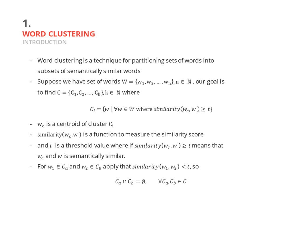
for partitioning sets of words into subsets of semantically similar words - Suppose we have set of words W = w$ ,w& , … , w( , n ∈ ℕ , our goal is to find C = C$ ,C& , …, C. , k ∈ ℕ where - w1 is a centroid of cluster C2 - similarity w1 ,w is a function to measure the similarity score - and is a threshold value where if D , ≥ means that D and is semantically similar. - For $ ∈ G and & ∈ H apply that $ , & < , so J = ∀ ∈ where D , ≥ } G ∩ H = ∅, ∀G ,H ∈
we need to: 1. Represent word as vector semantics, so we can compute their similarity and dissimilarity score. 2. Find the w1 for each cluster. 3. Choose the similarity metric D , and the threshold value .
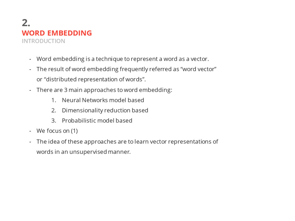
to represent a word as a vector. - The result of word embedding frequently referred as “word vector” or “distributed representation of words”. - There are 3 main approaches to word embedding: 1. Neural Networks model based 2. Dimensionality reduction based 3. Probabilistic model based - We focus on (1) - The idea of these approaches are to learn vector representations of words in an unsupervised manner.
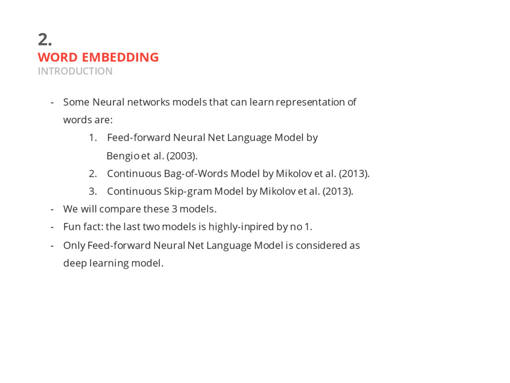
can learn representation of words are: 1. Feed-forward Neural Net Language Model by Bengio et al. (2003). 2. Continuous Bag-of-Words Model by Mikolov et al. (2013). 3. Continuous Skip-gram Model by Mikolov et al. (2013). - We will compare these 3 models. - Fun fact: the last two models is highly-inpired by no 1. - Only Feed-forward Neural Net Language Model is considered as deep learning model.
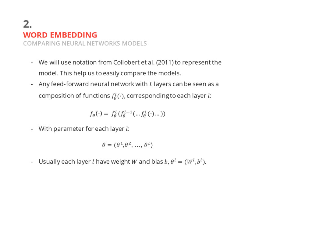
use notation from Collobert et al. (2011) to represent the model. This help us to easily compare the models. - Any feed-forward neural network with layers can be seen as a composition of functions T U(W), corresponding to each layer : - With parameter for each layer : - Usually each layer have weight and bias , U = (U,U). T W = T [ (T [\$(… T $(W)… )) = ($,&, …, [)
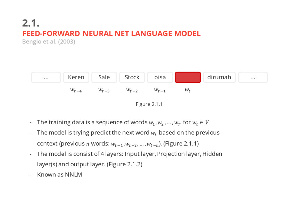
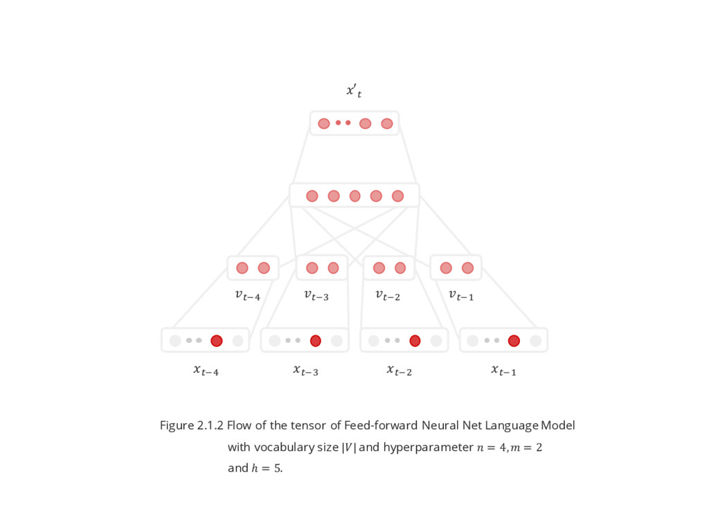
- The training data is a sequence of words $ , & , … , ] for ^ ∈ - The model is trying predict the next word ^ based on the previous context (previous words: ^ \$ ,^ \& , … , ^ \a ). (Figure 2.1.1) - The model is consist of 4 layers: Input layer, Projection layer, Hidden layer(s) and output layer. (Figure 2.1.2) - Known as NNLM ^ Keren Sale Stock bisa dirumah ... ... ^ \$ ^ \& ^ \b ^ \c Figure 2.1.1
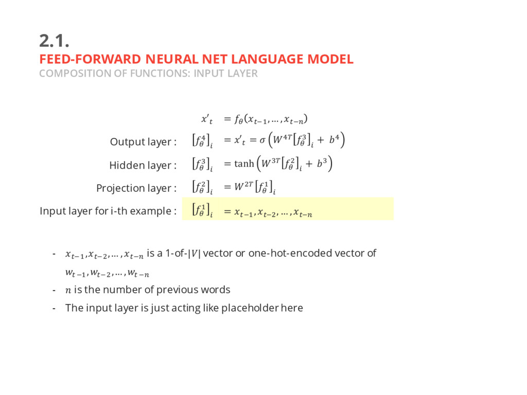
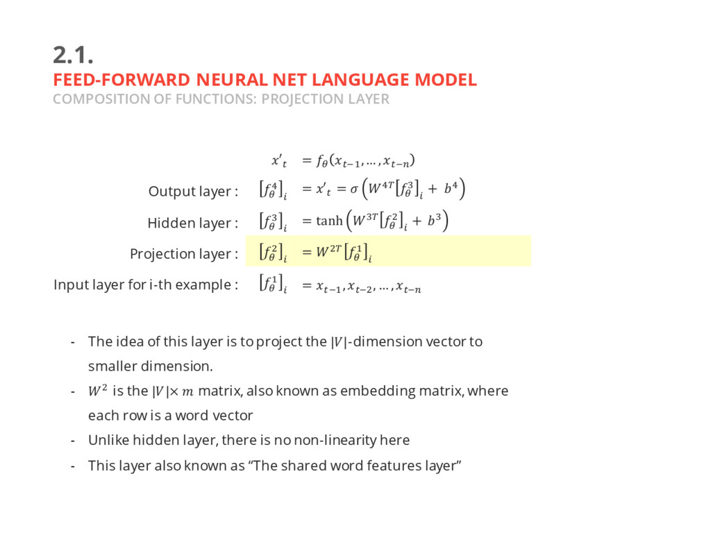
LAYER - ^\$ ,^\& ,… , ^\a is a 1-of-|| vector or one-hot-encoded vector of ^ \$ , ^\& ,… , ^ \a - is the number of previous words - The input layer is just acting like placeholder here ′^ = T ^\$ ,… , ^\a Output layer : T c J = ′^ = c] T b J + c Hidden layer : T b J = tanh b] T & J + b Projection layer : T & J = &] T $ J Input layer for i-th example : T $ J = ^\$ , ^\& , … , ^\a
LAYER - The idea of this layer is to project the ||-dimension vector to smaller dimension. - & is the ||× matrix, also known as embedding matrix, where each row is a word vector - Unlike hidden layer, there is no non-linearity here - This layer also known as “The shared word features layer” ′^ = T ^\$ ,… , ^\a Output layer : T c J = ′^ = c] T b J + c Hidden layer : T b J = tanh b] T & J + b Projection layer : T & J = &] T $ J Input layer for i-th example : T $ J = ^\$ , ^\& , … , ^\a
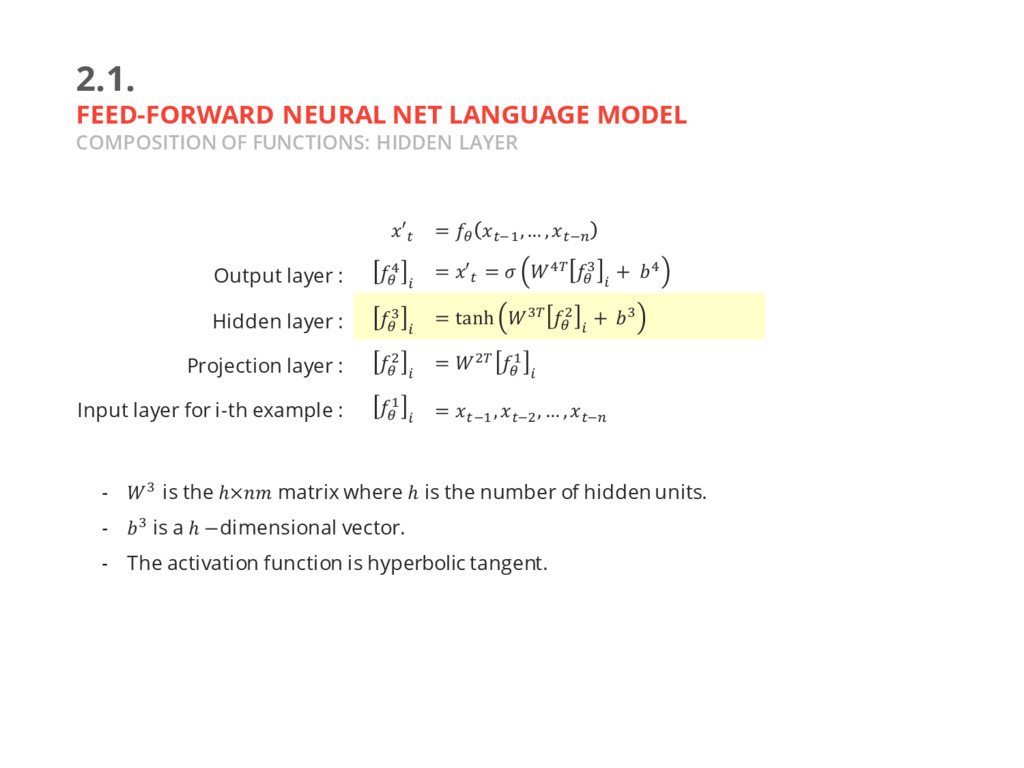
LAYER - b is the ℎ× matrix where ℎ is the number of hidden units. - b is a ℎ −dimensional vector. - The activation function is hyperbolic tangent. ′^ = T ^\$ ,… , ^\a Output layer : T c J = ′^ = c] T b J + c Hidden layer : T b J = tanh b] T & J + b Projection layer : T & J = &] T $ J Input layer for i-th example : T $ J = ^\$ , ^\& , … , ^\a
LAYER - c is the ℎ×|| matrix. - c is a ||-dimensional vector. - The activation function is softmax. - ′^ is a ||-dimensional vector. ′^ = T ^\$ ,… , ^\a Output layer : T c J = ′^ = c] T b J + c Hidden layer : T b J = tanh b] T & J + b Projection layer : T & J = &] T $ J Input layer for i-th example : T $ J = ^\$ , ^\& , … , ^\a
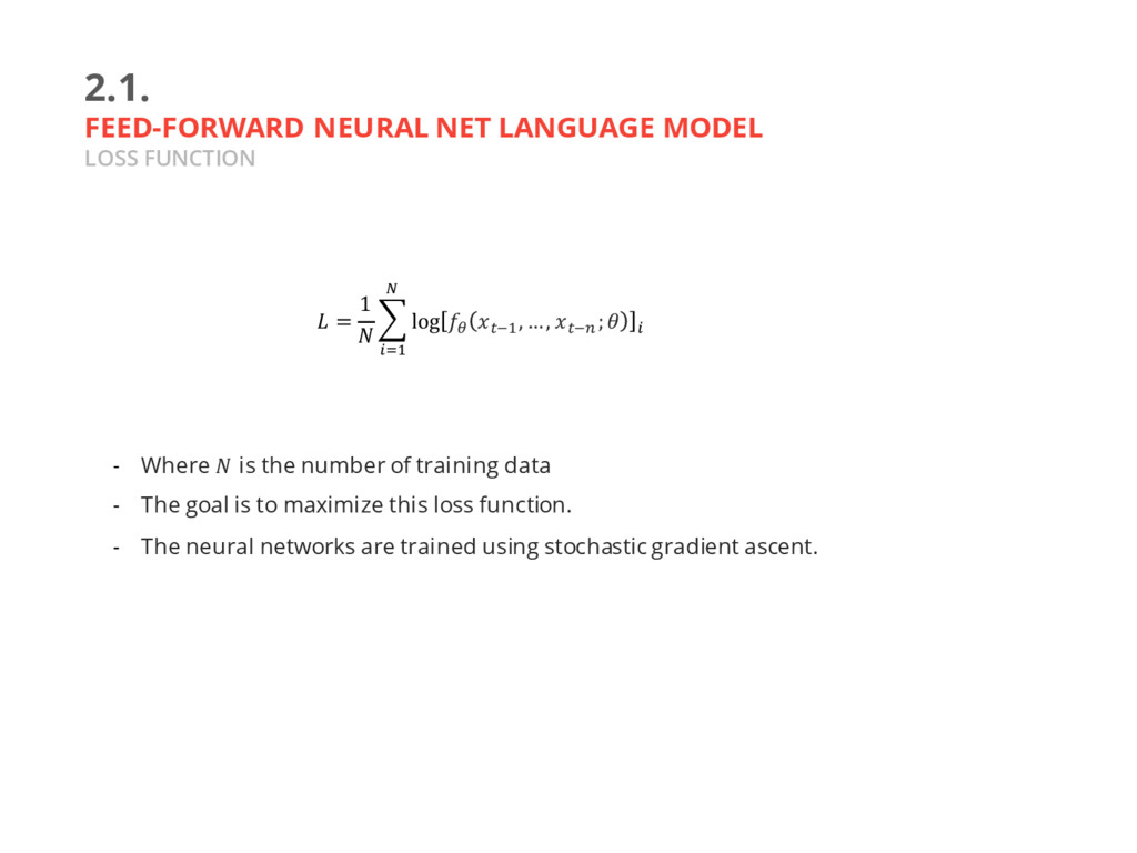
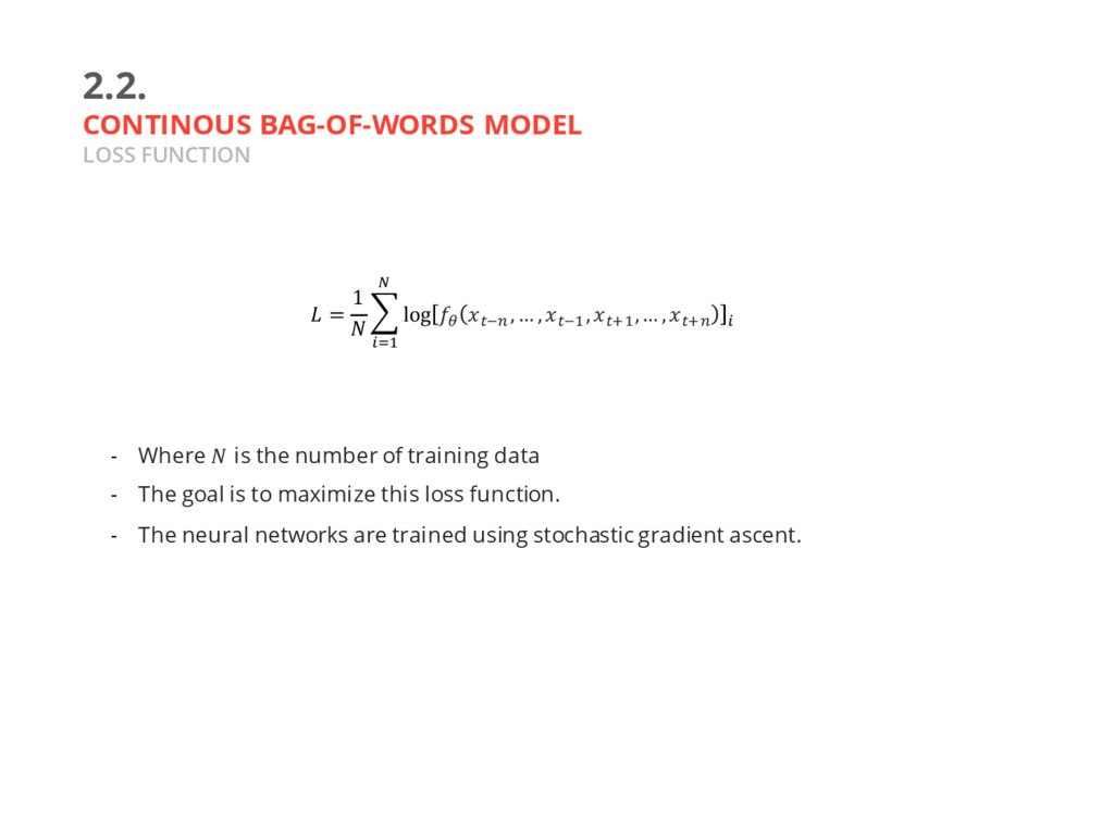
is the number of training data - The goal is to maximize this loss function. - The neural networks are trained using stochastic gradient ascent. = 1 n log T ^\$ , …, ^\a ; J r Js$
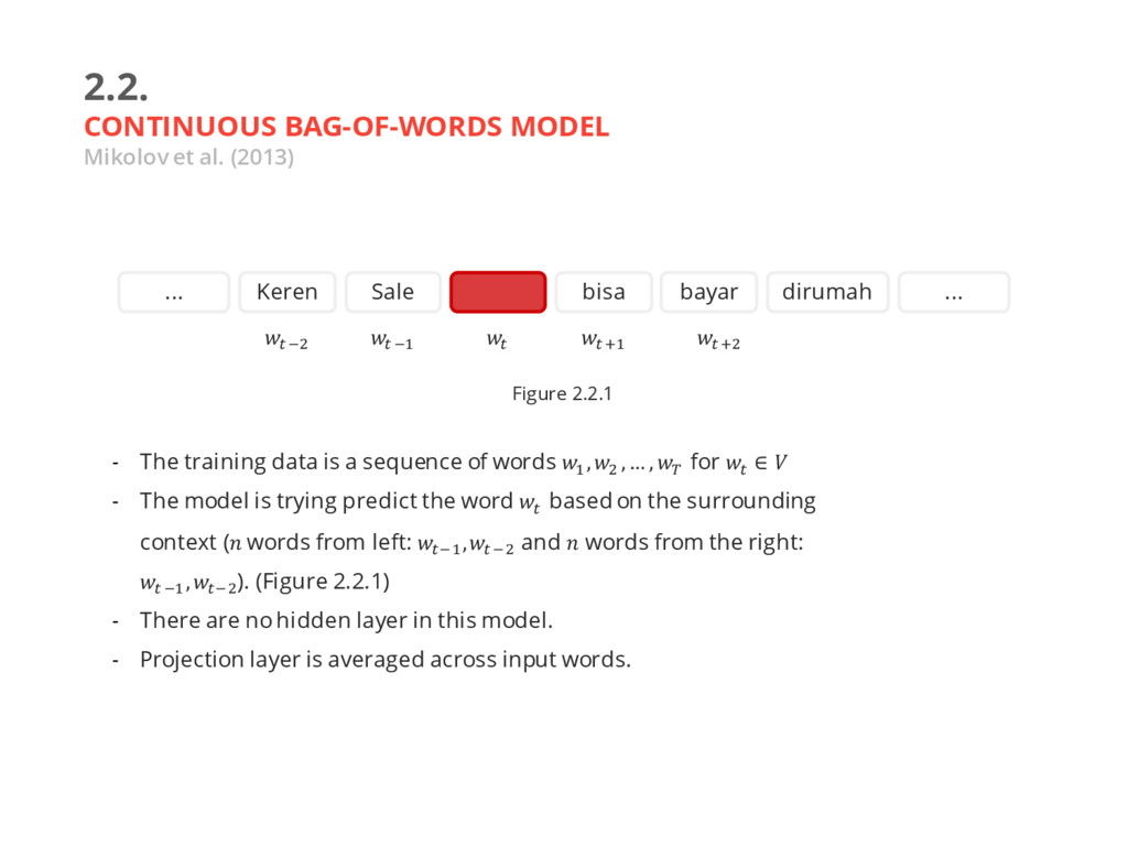
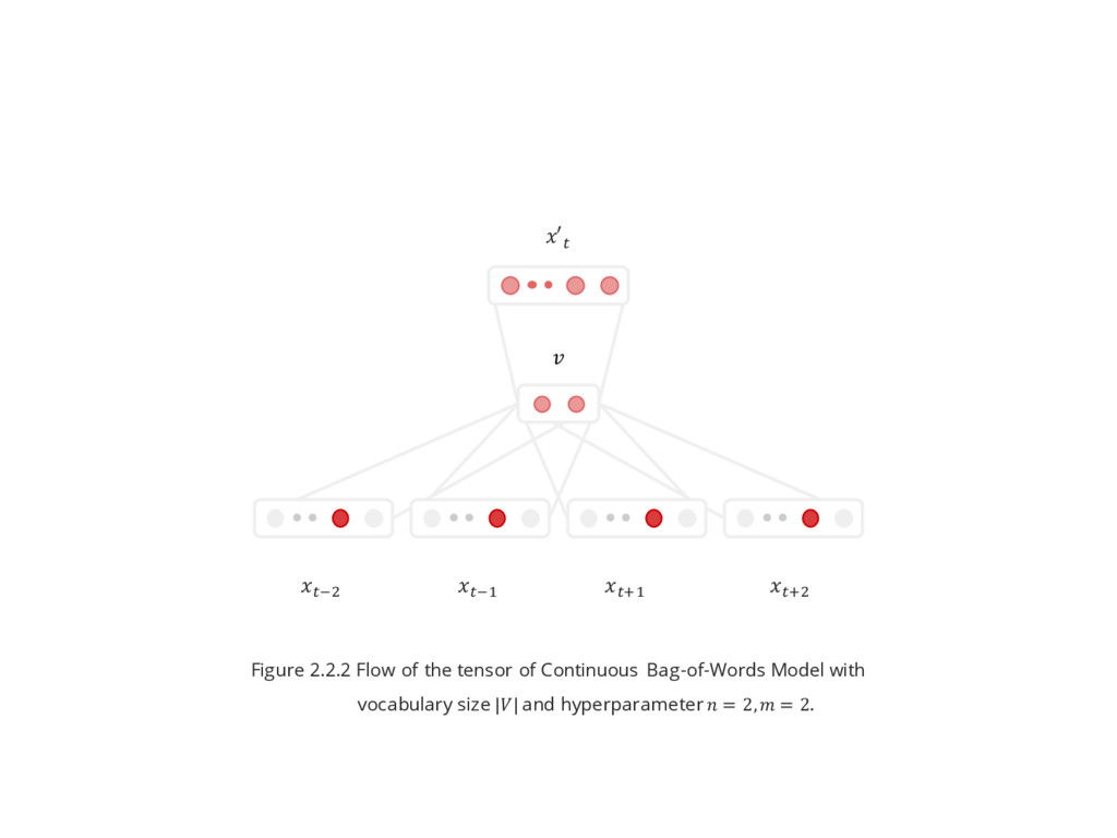
training data is a sequence of words $ , & , … , ] for ^ ∈ - The model is trying predict the word ^ based on the surrounding context ( words from left: ^\$ ,^ \& and words from the right: ^ \$ , ^\& ). (Figure 2.2.1) - There are no hidden layer in this model. - Projection layer is averaged across input words. ^ x& Keren Sale bisa bayar dirumah ... ... ^ x$ ^ ^ \$ ^ \& Figure 2.2.1
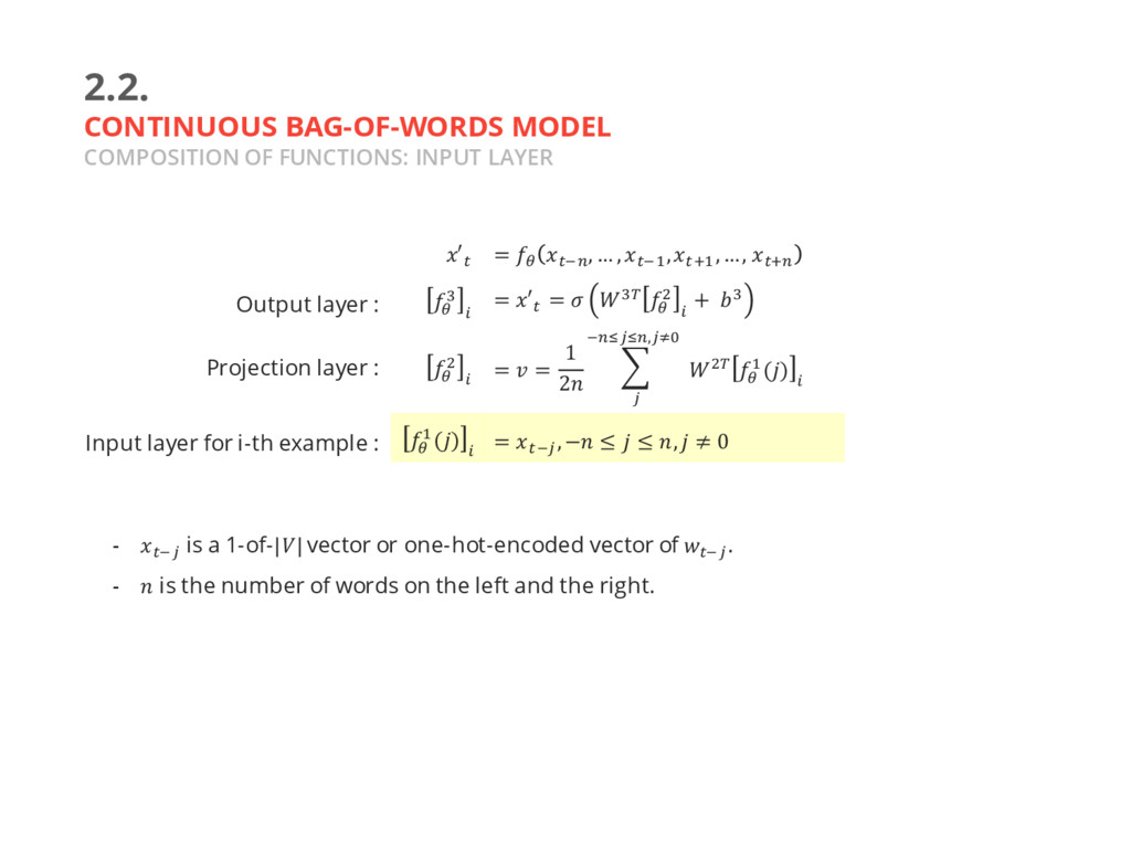
^\y is a 1-of-|| vector or one-hot-encoded vector of ^\y . - is the number of words on the left and the right. ′^ = T ^\a , … , ^\$ ,^x$ , …, ^xa Output layer : T b J = ′^ = b] T & J + b Projection layer : T & J = = 1 2 n &] T $() J \a{y{a,y|} y Input layer for i-th example : T $() J = ^\y , − ≤ ≤ , ≠ 0
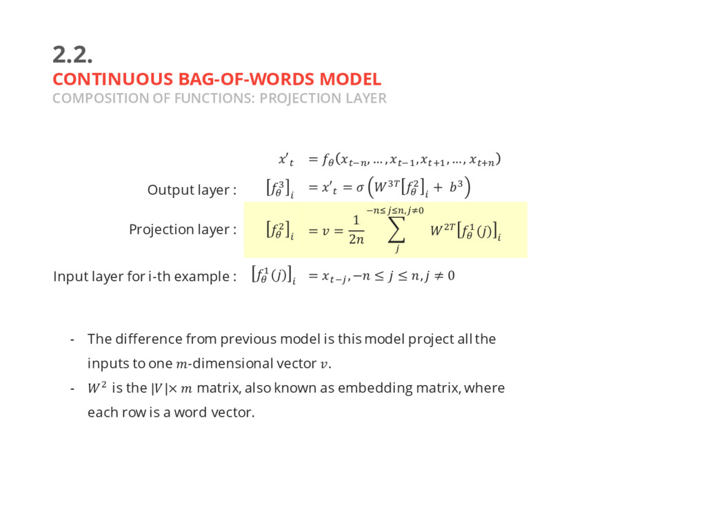
The difference from previous model is this model project all the inputs to one -dimensional vector . - & is the ||× matrix, also known as embedding matrix, where each row is a word vector. ′^ = T ^\a , … , ^\$ ,^x$ , …, ^xa Output layer : T b J = ′^ = b] T & J + b Projection layer : T & J = = 1 2 n &] T $() J \a{y{a,y|} y Input layer for i-th example : T $() J = ^\y , − ≤ ≤ , ≠ 0
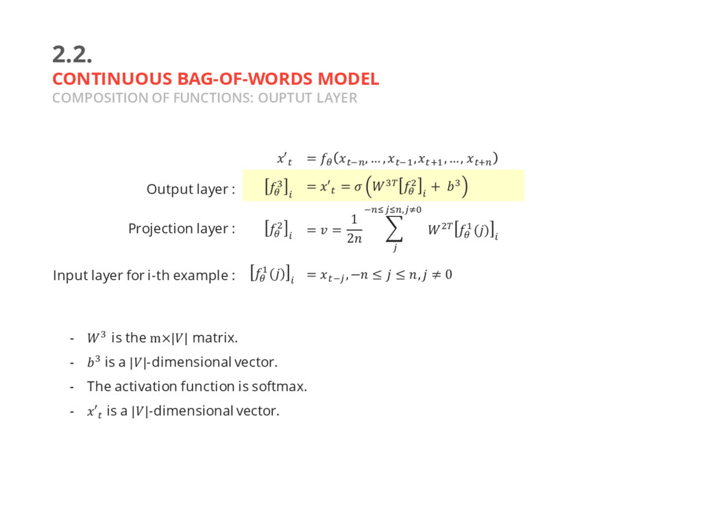
b is the m×|| matrix. - b is a ||-dimensional vector. - The activation function is softmax. - ′^ is a ||-dimensional vector. ′^ = T ^\a , … , ^\$ ,^x$ , …, ^xa Output layer : T b J = ′^ = b] T & J + b Projection layer : T & J = = 1 2 n &] T $() J \a{y{a,y|} y Input layer for i-th example : T $() J = ^\y , − ≤ ≤ , ≠ 0
number of training data - The goal is to maximize this loss function. - The neural networks are trained using stochastic gradient ascent. = 1 n log T ^\a , … , ^\$ , ^x$ ,… , ^xa J r Js$
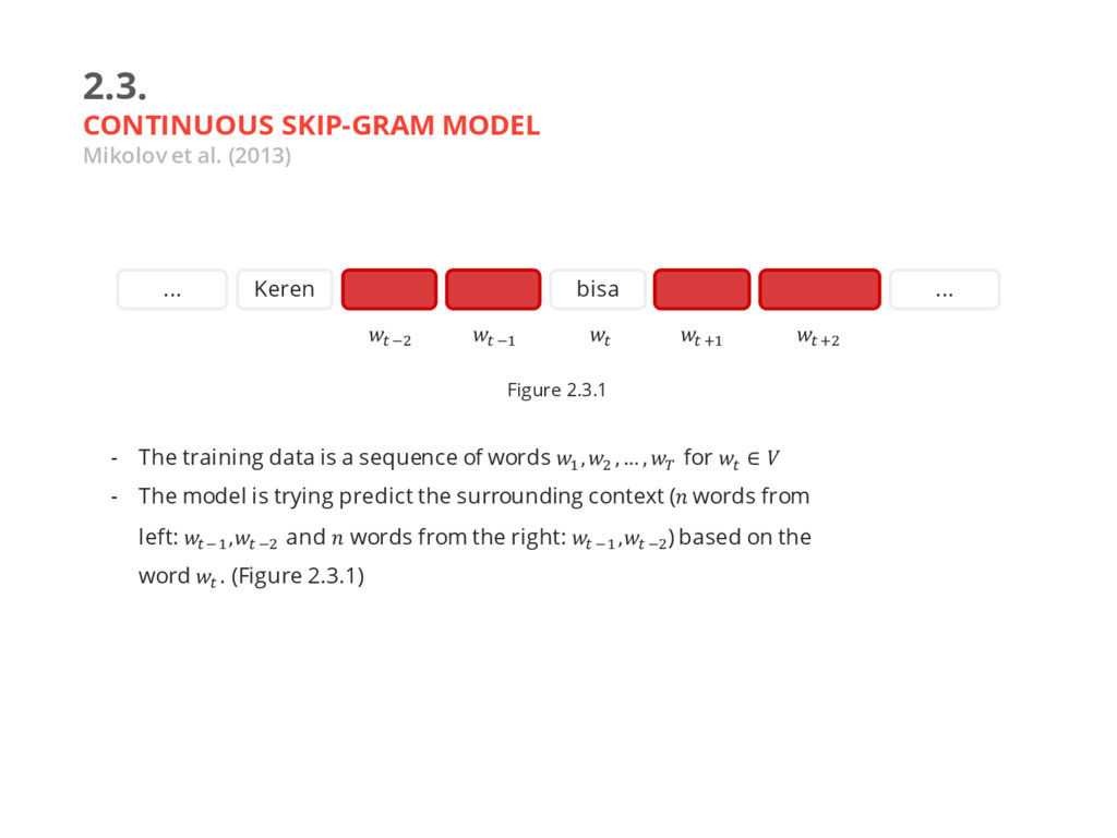
training data is a sequence of words $ , & , … , ] for ^ ∈ - The model is trying predict the surrounding context ( words from left: ^\$ ,^ \& and words from the right: ^ \$ ,^ \& ) based on the word ^ . (Figure 2.3.1) ^ x& Keren bisa ... ... ^ x$ ^ ^ \$ ^ \& Figure 2.3.1
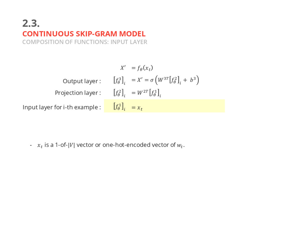
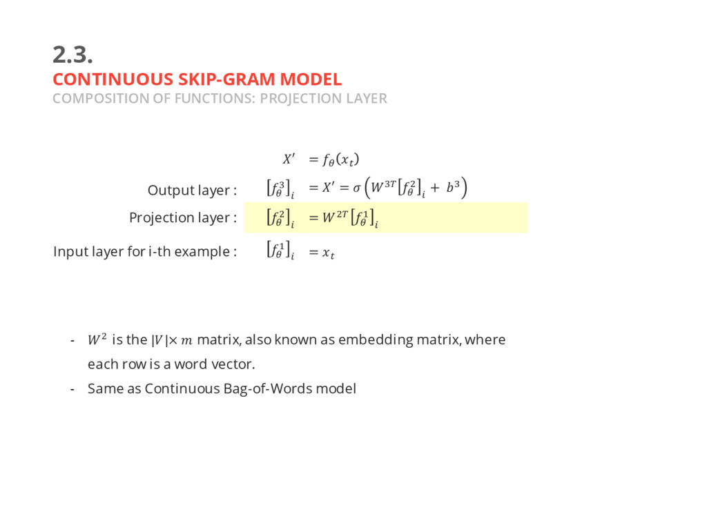
^ is a 1-of-|| vector or one-hot-encoded vector of ^ . ′ = T ^ Output layer : T b J = ′ = b] T & J + b Projection layer : T & J = &] T $ J Input layer for i-th example : T $ J = ^
& is the ||× matrix, also known as embedding matrix, where each row is a word vector. - Same as Continuous Bag-of-Words model ′ = T ^ Output layer : T b J = ′ = b] T & J + b Projection layer : T & J = &] T $ J Input layer for i-th example : T $ J = ^
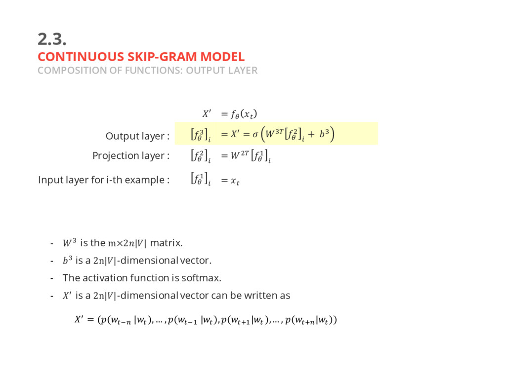
b is the m×2|| matrix. - b is a 2n||-dimensional vector. - The activation function is softmax. - ‚ is a 2n||-dimensional vector can be written as ′ = T ^ Output layer : T b J = ′ = b] T & J + b Projection layer : T & J = &] T $ J Input layer for i-th example : T $ J = ^ ‚ = ((^\a |^ ), … , (^\$ |^ ), (^x$ |^ ),… , (^xa |^ ))
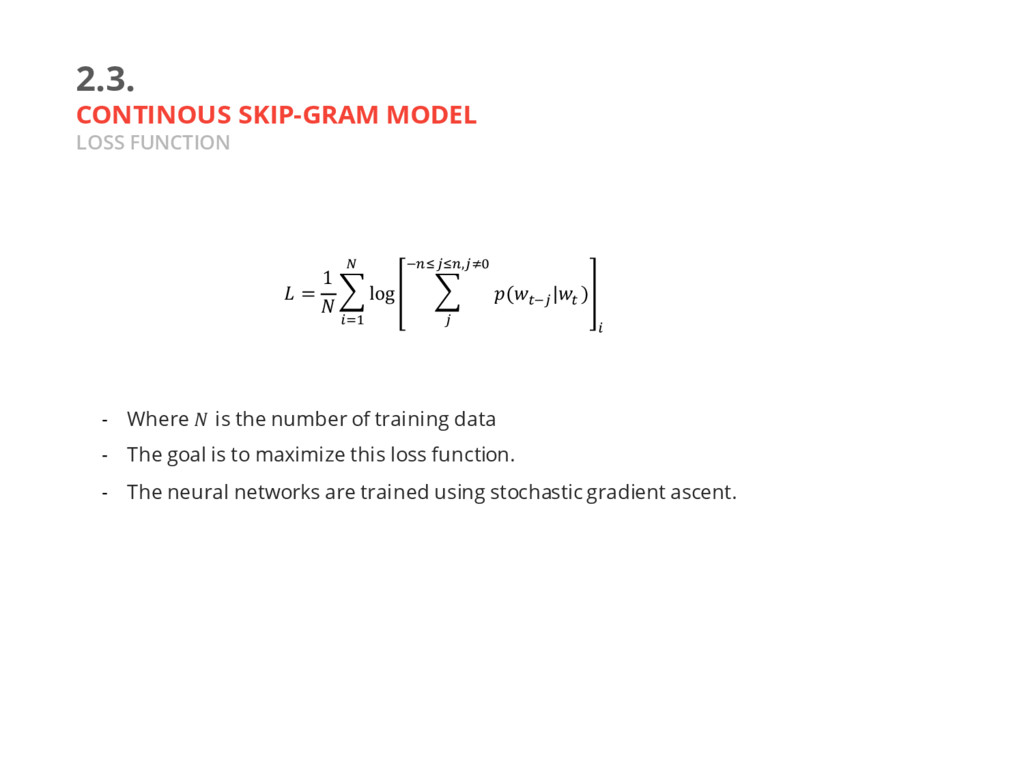
number of training data - The goal is to maximize this loss function. - The neural networks are trained using stochastic gradient ascent. = 1 n log n (^\y |^ ) \a{y{a,y|} y J r Js$
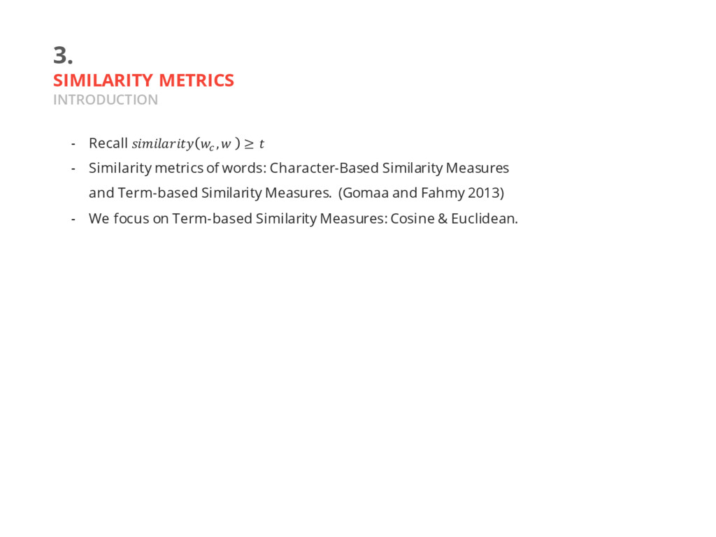
Similarity metrics of words: Character-Based Similarity Measures and Term-based Similarity Measures. (Gomaa and Fahmy 2013) - We focus on Term-based Similarity Measures
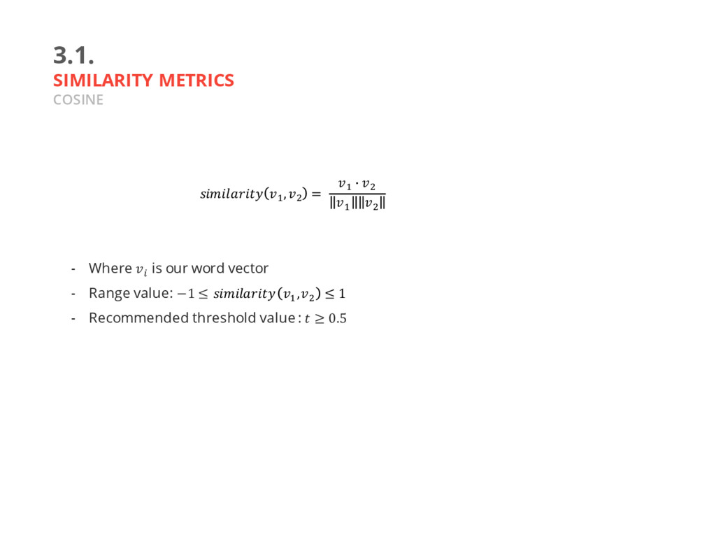
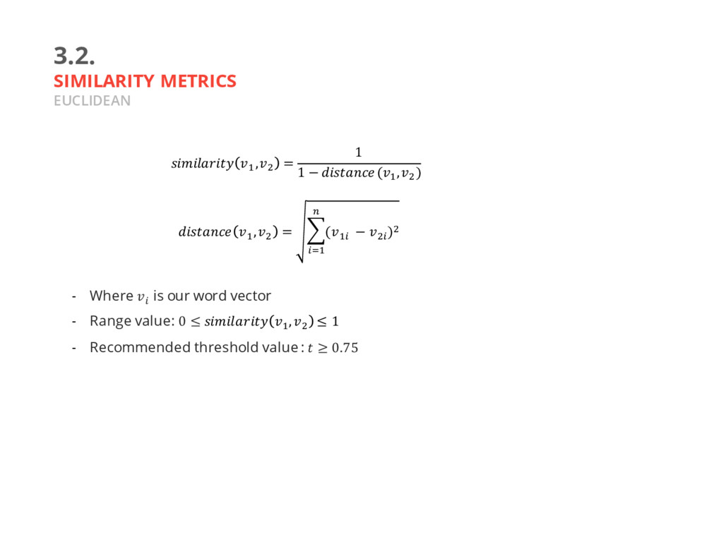
Similarity metrics of words: Character-Based Similarity Measures and Term-based Similarity Measures. (Gomaa and Fahmy 2013) - We focus on Term-based Similarity Measures: Cosine & Euclidean.
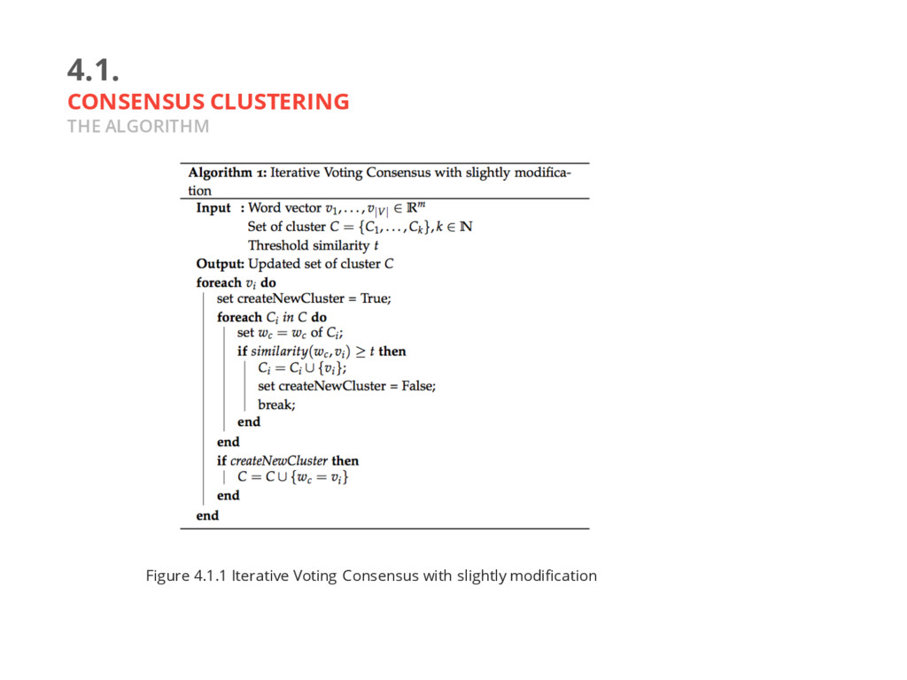
we want to find the D based on the consensus - There are 3 approaches for Consensus clustering: Iterative Voting Consensus, Iterative Probabilistic Voting Consensus and Iterative Pairwise Consensus. (Nguyen and Caruana 2007) - We use slightly modified version of Iterative Voting Consensus