Moving Mass, Decreasing Energy - Learning Probability Distributions with Wasserstein Gradient Flows

Talk held at the BMS-BGSMath Junior Meeting 2026 in Barcelona (https://www.crm.cat/bms-bgsmath-junior-meeting-2026/).

1. Moving Mass, Decreasing Energy Learning Probability Distributions with Wasserstein Gradient Flows Viktor Stein Technical University of Munich Munich Center for Machine Learning BMS–BGSMath Junior Meeting, 04.09.26
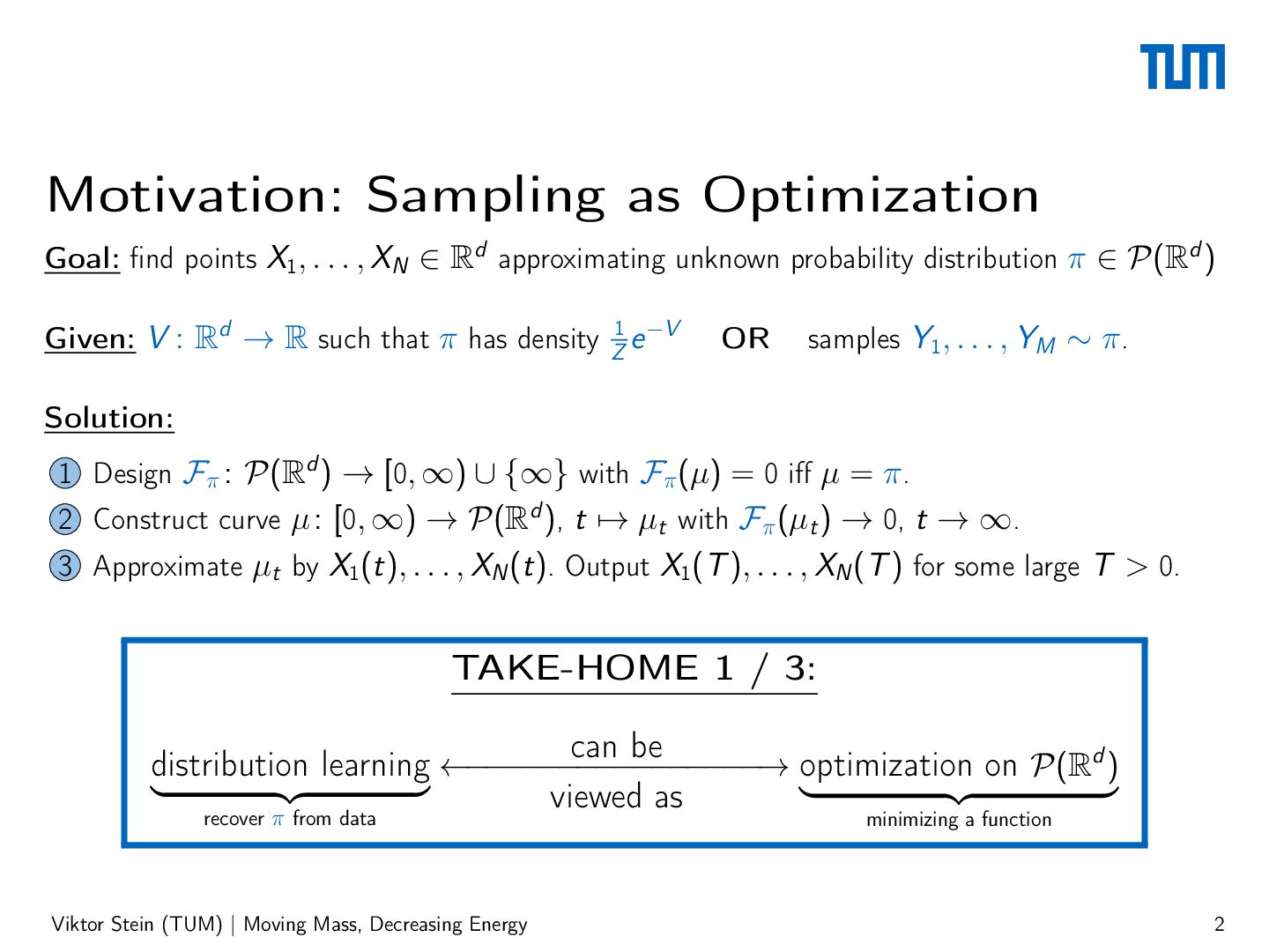
2. Motivation: Sampling as Optimization Goal: find points X1, . . . , XN ∈ Rd approximating unknown probability distribution π ∈ P(Rd ) Given: V : Rd → R such that π has density Z1 e −V OR samples Y1, . . . , YM ∼ π . Solution: 1 Design Fπ : P(Rd ) → [0, ∞) ∪ {∞} with Fπ (µ) = 0 iff µ = π . 2 Construct curve µ : [0, ∞) → P(Rd ), t ↦→ µt with Fπ (µt ) → 0, t → ∞. 3 Approximate µt by X1(t), . . . , XN (t). Output X1(T ), . . . , XN (T ) for some large T > 0. TAKE-HOME 1 / 3: can be distribution learning ←−−−−−−−−−−−−−−−−→ optimization on P(Rd ) ⏞ ⏟⏟ ⏞ ⏟⏟ ⏞ ⏞ viewed as recover π from data minimizing a function Viktor Stein (TUM) | Moving Mass, Decreasing Energy 2
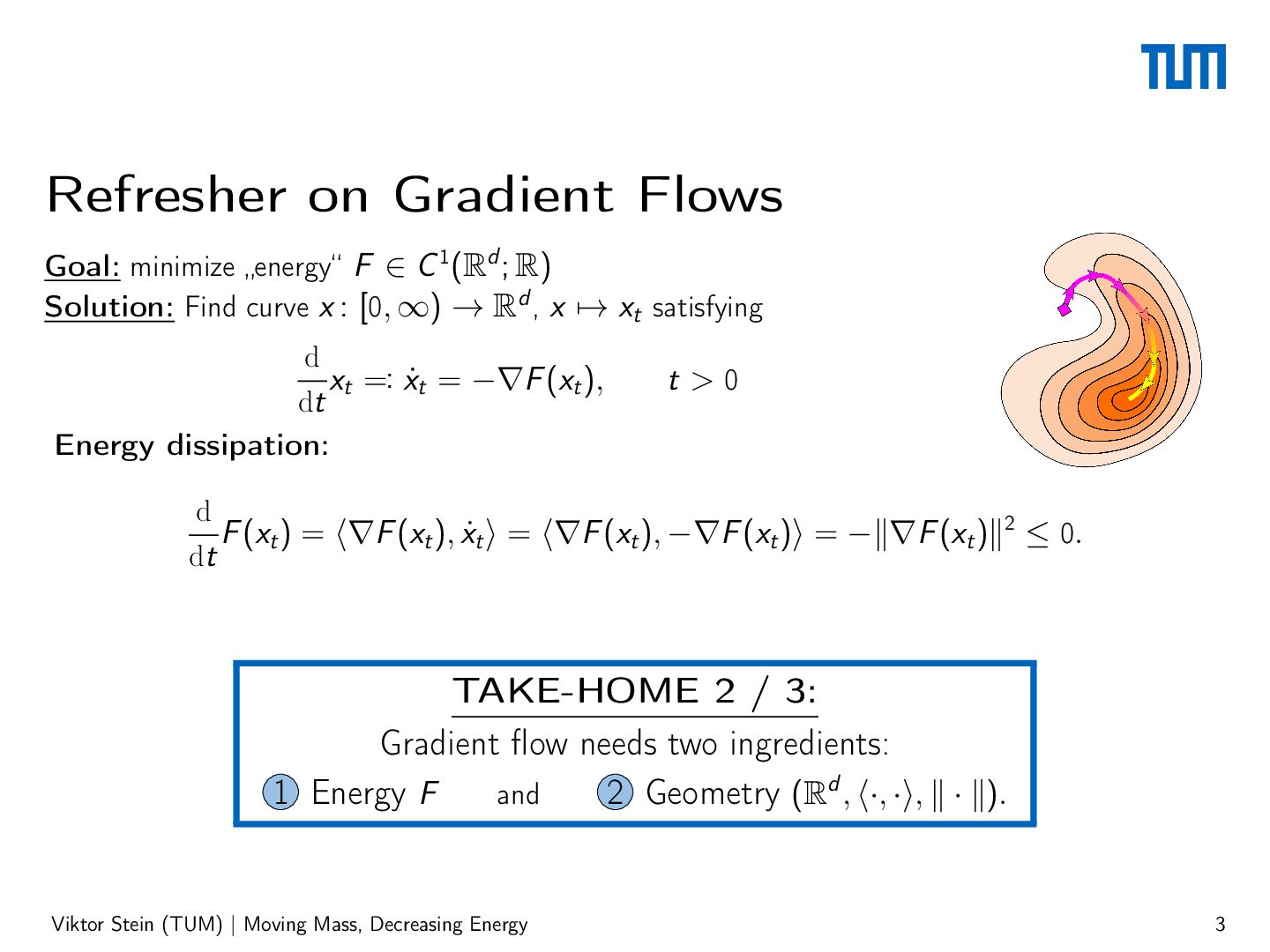
3. Refresher on Gradient Flows Goal: minimize „energy“ F ∈ C 1(Rd ; R) Solution: Find curve x : [0, ∞) → Rd , x ↦→ xt satisfying d xt =: ẋt = −∇F (xt ), dt Energy dissipation: t>0 d F (xt ) = ⟨∇F (xt ), ẋt ⟩ = ⟨∇F (xt ), −∇F (xt )⟩ = −∥∇F (xt )∥2 ≤ 0. dt TAKE-HOME 2 / 3: Gradient flow needs two ingredients: 1 Energy F and 2 Geometry (Rd , ⟨·, ·⟩, ∥ · ∥). Viktor Stein (TUM) | Moving Mass, Decreasing Energy 3
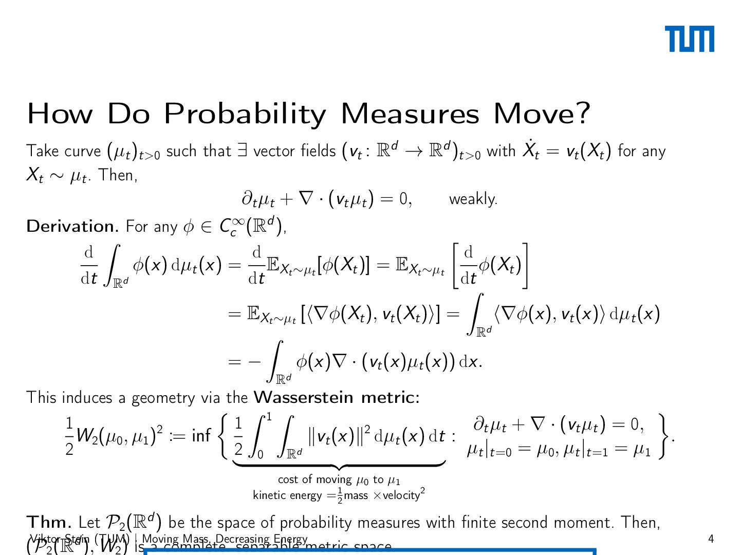
4. How Do Probability Measures Move? Take curve (µt )t>0 such that ∃ vector fields (vt : Rd → Rd )t>0 with Ẋt = vt (Xt ) for any Xt ∼ µt . Then, ∂t µt + ∇ · (vt µt ) = 0, weakly. Derivation. For any ϕ ∈ Cc∞(Rd ), [︃ ]︃ ∫︂ d d d ϕ(x) dµt (x) = EXt ∼µt [ϕ(Xt )] = EXt ∼µt ϕ(Xt ) dt Rd dt dt ∫︂ = EXt ∼µt [⟨∇ϕ(Xt ), vt (Xt )⟩] = ⟨∇ϕ(x), vt (x)⟩ dµt (x) d R ∫︂ =− ϕ(x)∇ · (vt (x)µt (x)) dx. Rd This induces a geometry via the Wasserstein metric: {︃ ∫︂ 1 ∫︂ }︃ 1 1 ∂ µ + ∇ · (vt µt ) = 0, W2(µ0, µ1)2 := inf ∥vt (x)∥2 dµt (x) dt : t t . µt |t=0 = µ0, µt |t=1 = µ1 2 2 0 Rd ⏞ ⏟⏟ cost of moving µ0 to µ1 kinetic energy = 21 mass ×velocity2 ⏞ Thm. Let P2(Rd ) be the space of probability measures with finite second moment. Then, Viktor Stein d (TUM) | Moving Mass, Decreasing Energy (P 2 (R ), W2 ) is a complete, separable metric space. 4
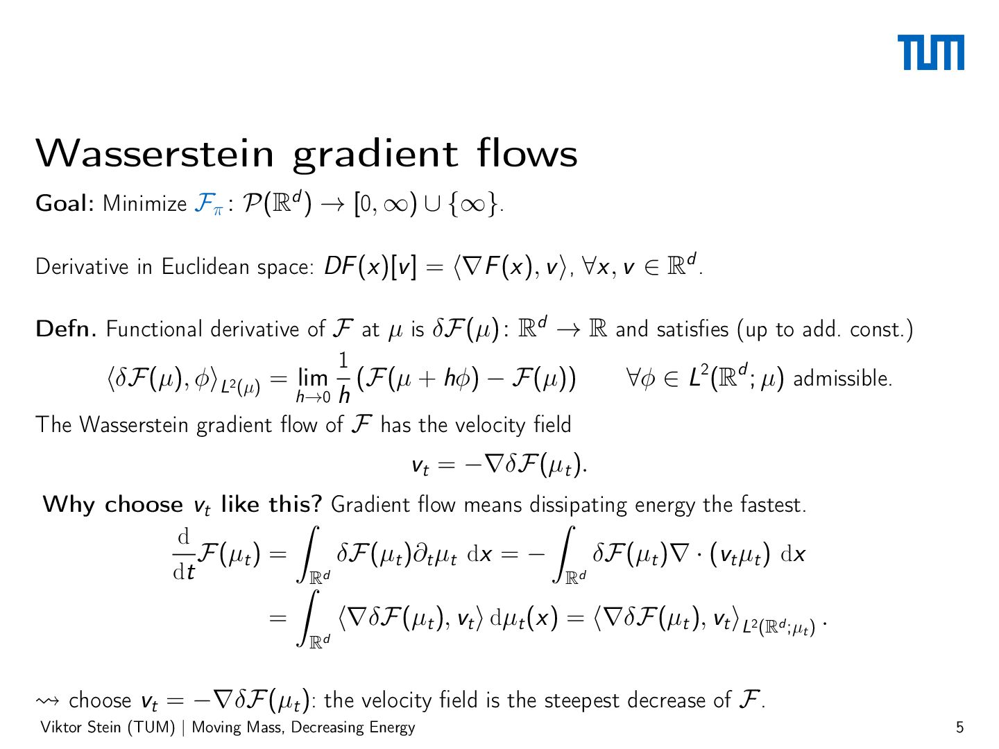
5. Wasserstein gradient flows Goal: Minimize Fπ : P(Rd ) → [0, ∞) ∪ {∞}. Derivative in Euclidean space: DF (x)[v ] = ⟨∇F (x), v ⟩, ∀x, v ∈ Rd . Defn. Functional derivative of F at µ is δF(µ) : Rd → R and satisfies (up to add. const.) 1 ∀ϕ ∈ L2(Rd ; µ) admissible. ⟨δF(µ), ϕ⟩L2(µ) = lim (F(µ + hϕ) − F(µ)) h→0 h The Wasserstein gradient flow of F has the velocity field vt = −∇δF(µt ). Why choose vt like this? Gradient flow means dissipating energy the fastest. ∫︂ ∫︂ d δF(µt )∂t µt dx = − δF(µt )∇ · (vt µt ) dx F(µt ) = dt d d R ∫︂R = Rd ⟨∇δF(µt ), vt ⟩ dµt (x) = ⟨∇δF(µt ), vt ⟩L2(Rd ;µt ) . ⇝ choose vt = −∇δF (µt ): the velocity field is the steepest decrease of F . Viktor Stein (TUM) | Moving Mass, Decreasing Energy 5
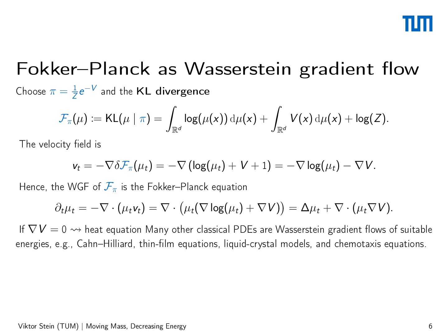
6. Fokker–Planck as Wasserstein gradient flow Choose π = Z1 e −V and the KL divergence ∫︂ Fπ (µ) := KL(µ | π) = ∫︂ log(µ(x)) dµ(x) + Rd V (x) dµ(x) + log(Z ). Rd The velocity field is vt = −∇δFπ (µt ) = −∇ (log(µt ) + V + 1) = −∇ log(µt ) − ∇V . Hence, the WGF of Fπ is the Fokker–Planck equation (︁ )︁ ∂t µt = −∇ · (µt vt ) = ∇ · µt (∇ log(µt ) + ∇V ) = ∆µt + ∇ · (µt ∇V ). If ∇V = 0 ⇝ heat equation Many other classical PDEs are Wasserstein gradient flows of suitable energies, e.g., Cahn–Hilliard, thin-film equations, liquid-crystal models, and chemotaxis equations. Viktor Stein (TUM) | Moving Mass, Decreasing Energy 6
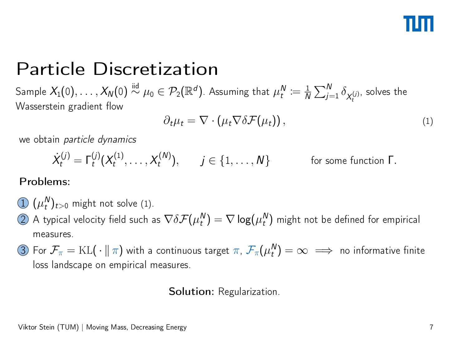
7. Particle Discretization iid 1 Sample X1(0), . . . , XN (0) ∼ µ0 ∈ P2(R ). Assuming that µN t := N d Wasserstein gradient flow ∑︁N j=1 δXt(j) , solves the ∂t µt = ∇ · (µt ∇δF (µt )) , (1) we obtain particle dynamics (j) (j) (1) (N) Ẋt = Γt (Xt , . . . , Xt ), j ∈ {1, . . . , N} for some function Γ. Problems: 1 (µN t )t>0 might not solve (1). N 2 A typical velocity field such as ∇δF(µN t ) = ∇ log(µt ) might not be defined for empirical measures. 3 For Fπ = KL( · ∥ π) with a continuous target π , Fπ (µN t ) = ∞ =⇒ no informative finite loss landscape on empirical measures. Solution: Regularization. Viktor Stein (TUM) | Moving Mass, Decreasing Energy 7
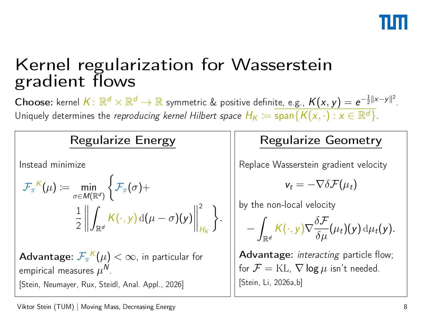
8. Kernel regularization for Wasserstein gradient flows 1 2 Choose: kernel K : Rd × Rd → R symmetric & positive definite, e.g., K (x, y ) = e − 2 ∥x−y ∥ . Uniquely determines the reproducing kernel Hilbert space HK := span{K (x, ·) : x ∈ Rd }. Regularize Energy Regularize Geometry Instead minimize Fπ K (µ) := Replace Wasserstein gradient velocity {︃ min Fπ (σ)+ σ∈M(Rd ) ⃦2 }︃ ⃦∫︂ ⃦ ⃦ 1⃦ K (·, y ) d(µ − σ)(y )⃦ . ⃦ ⃦ 2 d R HK vt = −∇δF(µt ) by the non-local velocity ∫︂ − K (·, y )∇ Rd δF (µt )(y ) dµt (y ). δµ Advantage: Fπ K (µ) < ∞, in particular for empirical measures µN . Advantage: interacting particle flow; for F = KL, ∇ log µ isn’t needed. [Stein, Neumayer, Rux, Steidl, Anal. Appl., 2026] [Stein, Li, 2026a,b] Viktor Stein (TUM) | Moving Mass, Decreasing Energy 8
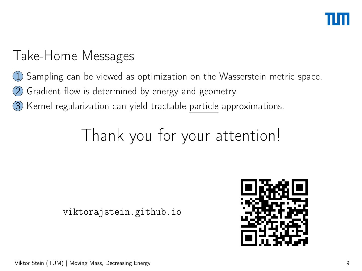
9. Take-Home Messages 1 Sampling can be viewed as optimization on the Wasserstein metric space. 2 Gradient flow is determined by energy and geometry. 3 Kernel regularization can yield tractable particle approximations. Thank you for your attention! viktorajstein.github.io Viktor Stein (TUM) | Moving Mass, Decreasing Energy 9