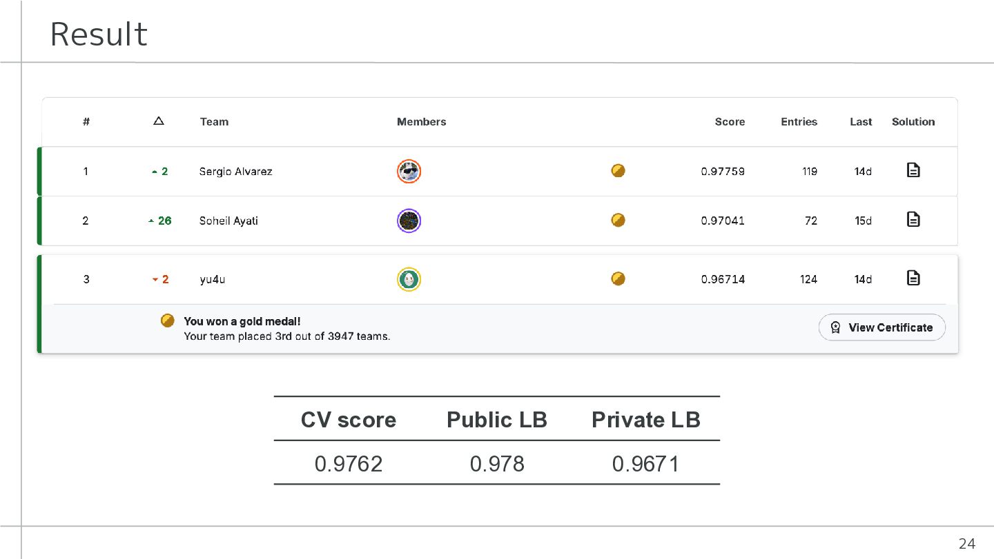
Biohub - Cell Tracking During Development: 3rd Place Solution

An overview of my 3rd-place solution to the Kaggle “Biohub – Cell Tracking During Development” competition, presented at the winners’ call.

The presentation covers a pipeline for tracking cells and reconstructing cell lineages in 3D time-lapse microscopy, with a focus on learning from sparse annotations. The approach combines 2.5D and 3D cell detection, self-supervised dense flow estimation, cell matching, and division identification, integrating their predictions through graph optimization. It also includes ablation studies examining how these components contribute to the final system.

Source code:
https://github.com/yu4u/kaggle-biohub-3rd

Technical paper: “Learning to Track Cells from Sparse Annotations in 3D Time-Lapse Microscopy”
https://arxiv.org/abs/2611.06624

Transcript

1. Biohub - Cell Tracking During Development 3rd Place Solution @yu4u
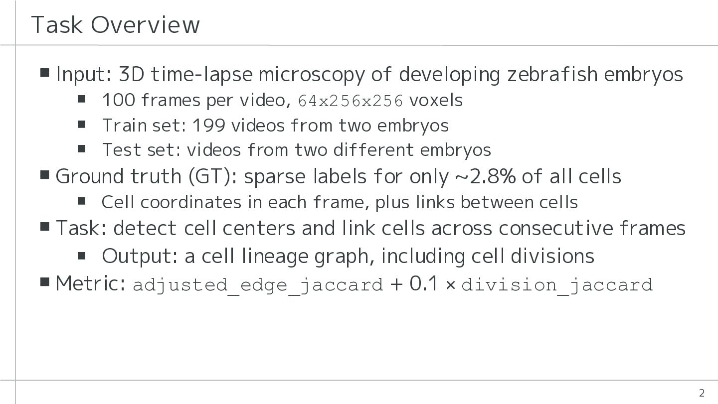
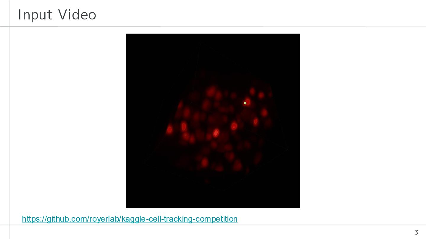
2. Task Overview ▪ Input: 3D time-lapse microscopy of developing zebrafish embryos ▪ 100 frames per video, 64x256x256 voxels ▪ Train set: 199 videos from two embryos ▪ Test set: videos from two different embryos ▪ Ground truth (GT): sparse labels for only ~2.8% of all cells ▪ Cell coordinates in each frame, plus links between cells ▪ Task: detect cell centers and link cells across consecutive frames ▪ Output: a cell lineage graph, including cell divisions ▪ Metric: adjusted_edge_jaccard + 0.1 × division_jaccard 2
3. Input Video https://github.com/royerlab/kaggle-cell-tracking-competition 3
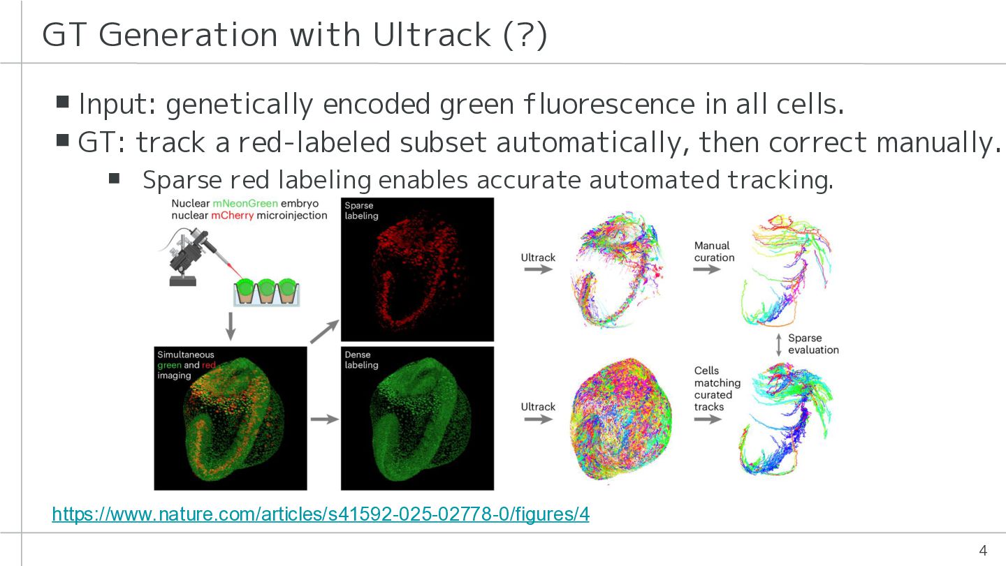
4. GT Generation with Ultrack (?) ▪ Input: genetically encoded green fluorescence in all cells. ▪ GT: track a red-labeled subset automatically, then correct manually. ▪ Sparse red labeling enables accurate automated tracking. https://www.nature.com/articles/s41592-025-02778-0/figures/4 4
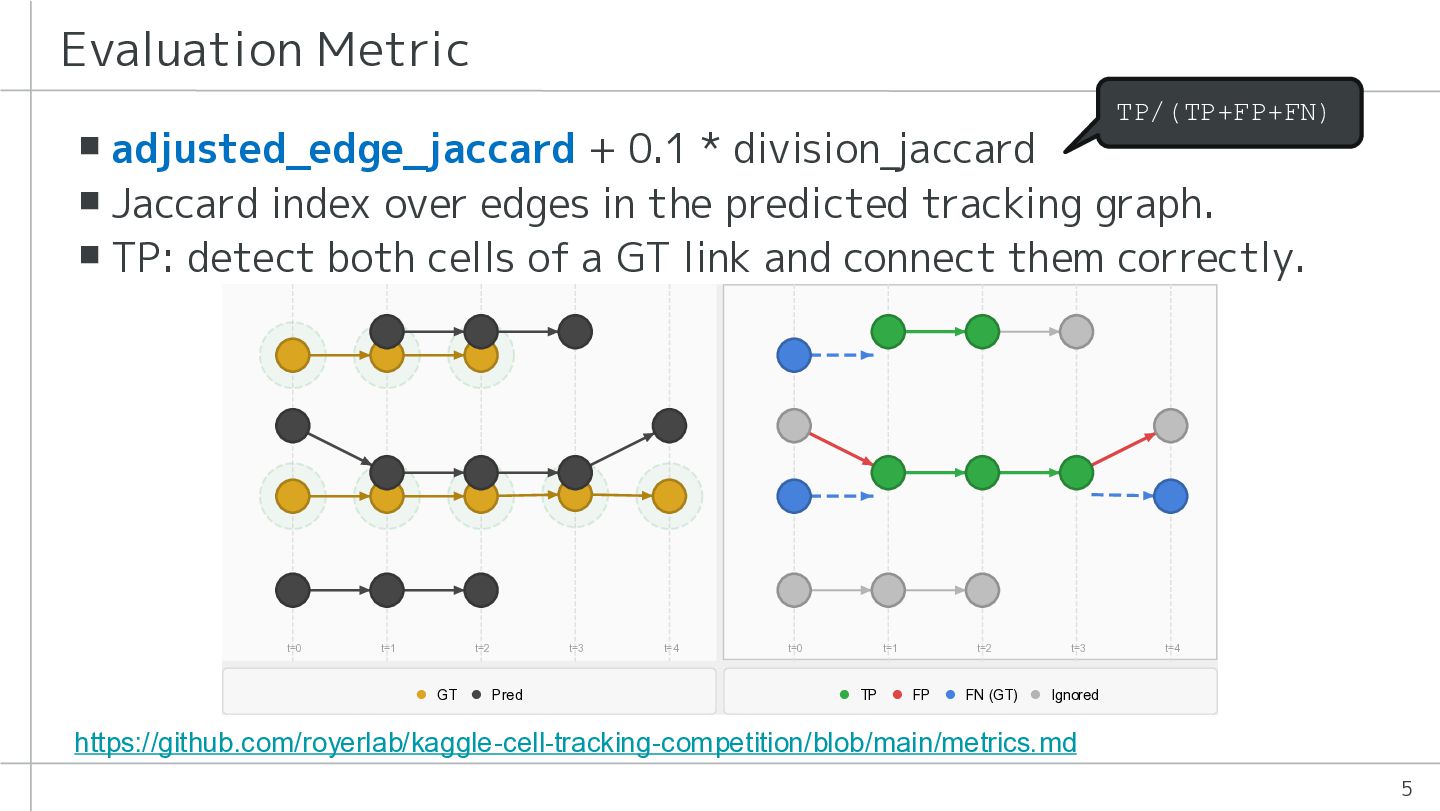
5. Evaluation Metric TP/(TP+FP+FN) ▪ adjusted_edge_jaccard + 0.1 * division_jaccard ▪ Jaccard index over edges in the predicted tracking graph. ▪ TP: detect both cells of a GT link and connect them correctly. https://github.com/royerlab/kaggle-cell-tracking-competition/blob/main/metrics.md 5
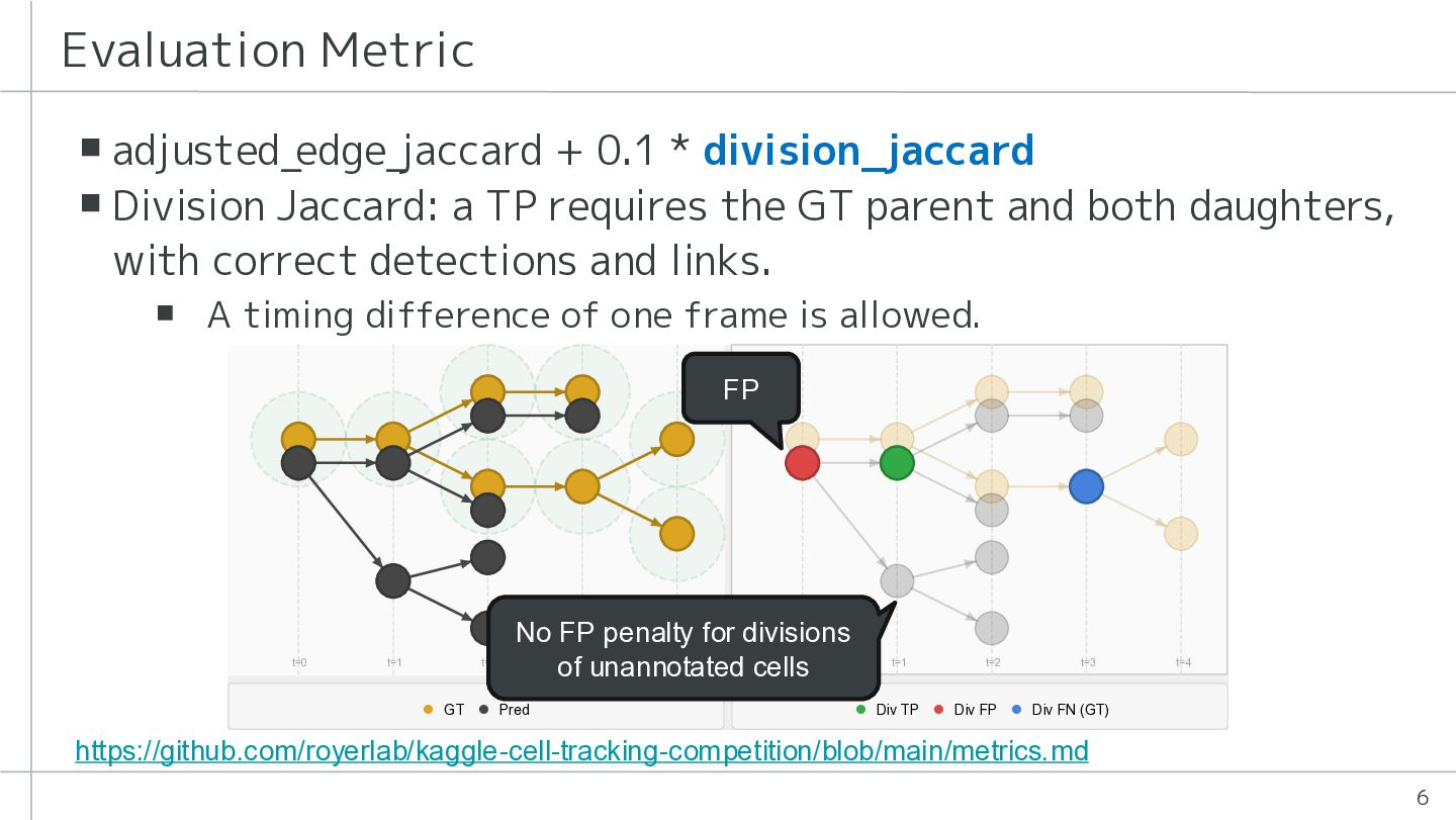
6. Evaluation Metric ▪ adjusted_edge_jaccard + 0.1 * division_jaccard ▪ Division Jaccard: a TP requires the GT parent and both daughters, with correct detections and links. ▪ A timing difference of one frame is allowed. FP No FP penalty for divisions of unannotated cells https://github.com/royerlab/kaggle-cell-tracking-competition/blob/main/metrics.md 6
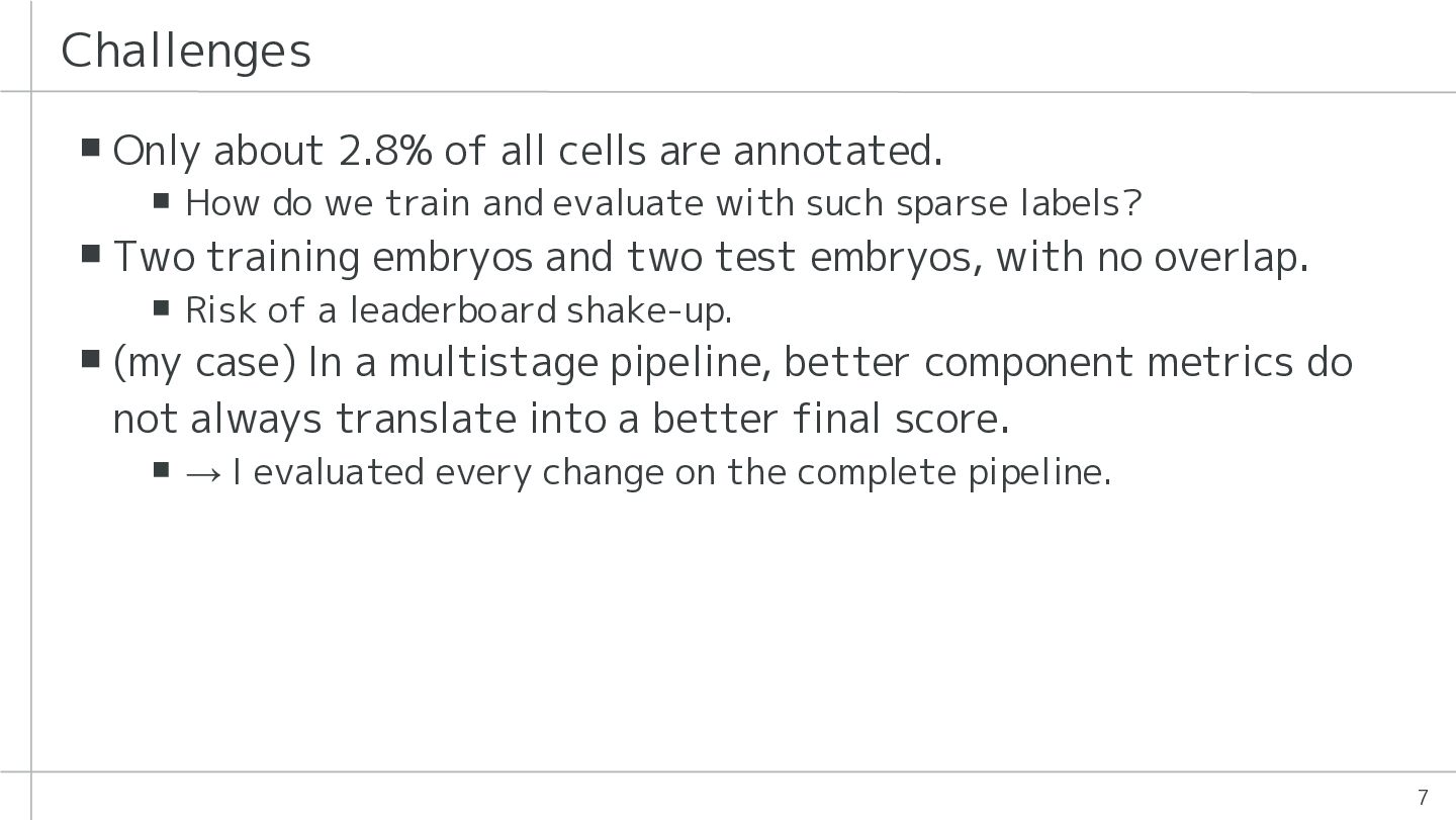
7. Challenges ▪ Only about 2.8% of all cells are annotated. ▪ How do we train and evaluate with such sparse labels? ▪ Two training embryos and two test embryos, with no overlap. ▪ Risk of a leaderboard shake-up. ▪ (my case) In a multistage pipeline, better component metrics do not always translate into a better final score. ▪ → I evaluated every change on the complete pipeline. 7
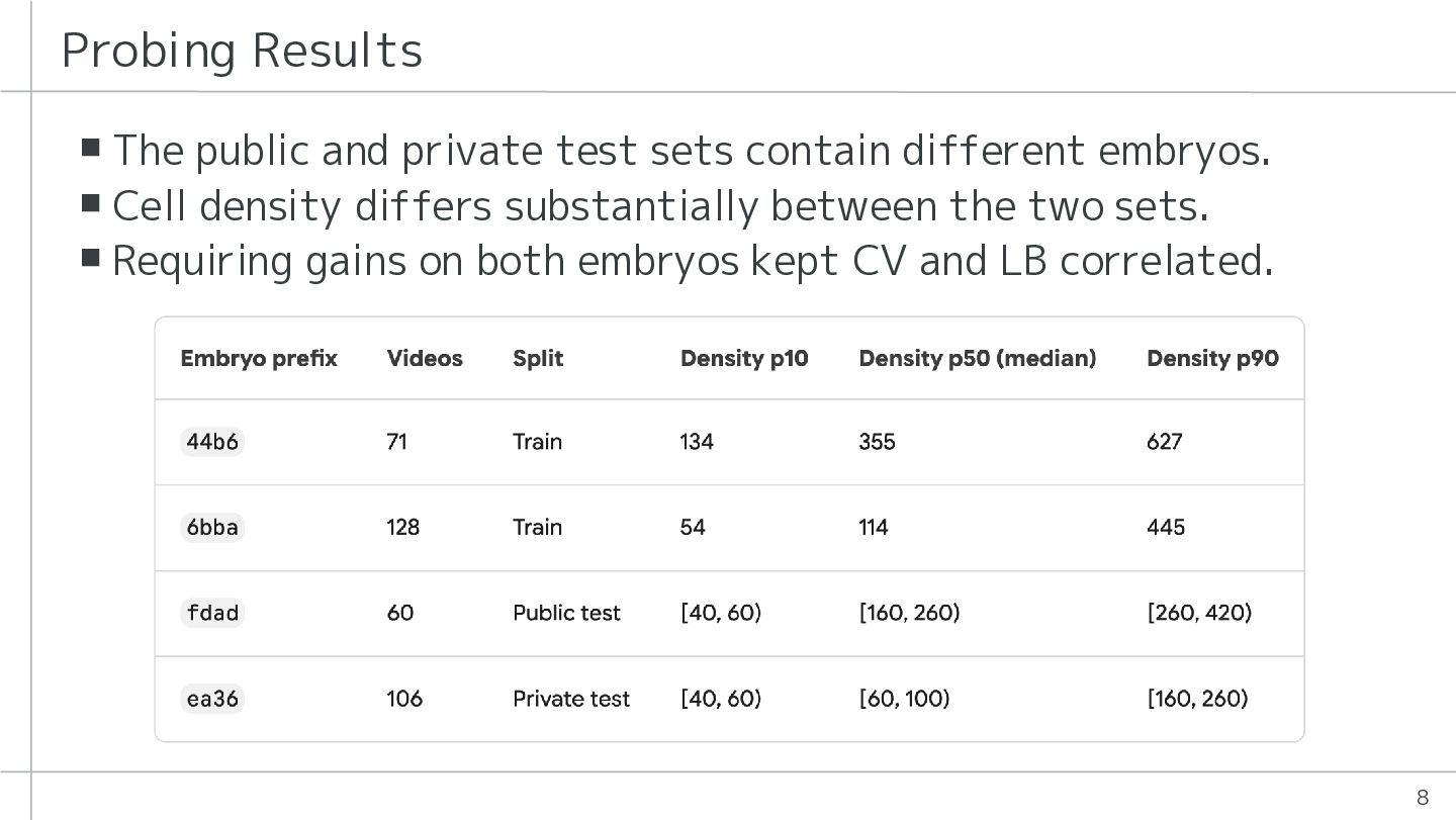
8. Probing Results ▪ The public and private test sets contain different embryos. ▪ Cell density differs substantially between the two sets. ▪ Requiring gains on both embryos kept CV and LB correlated. 8
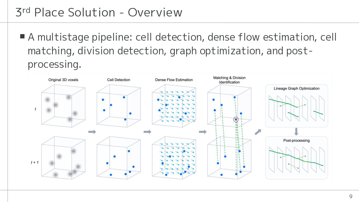
9. 3rd Place Solution - Overview ▪ A multistage pipeline: cell detection, dense flow estimation, cell matching, division detection, graph optimization, and postprocessing. 9
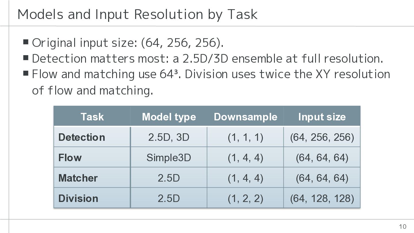
10. Models and Input Resolution by Task ▪ Original input size: (64, 256, 256). ▪ Detection matters most: a 2.5D/3D ensemble at full resolution. ▪ Flow and matching use 64³. Division uses twice the XY resolution of flow and matching. Task Model type Downsample Input size Detection 2.5D, 3D (1, 1, 1) (64, 256, 256) Flow Simple3D (1, 4, 4) (64, 64, 64) Matcher 2.5D (1, 4, 4) (64, 64, 64) Division 2.5D (1, 2, 2) (64, 128, 128) 10
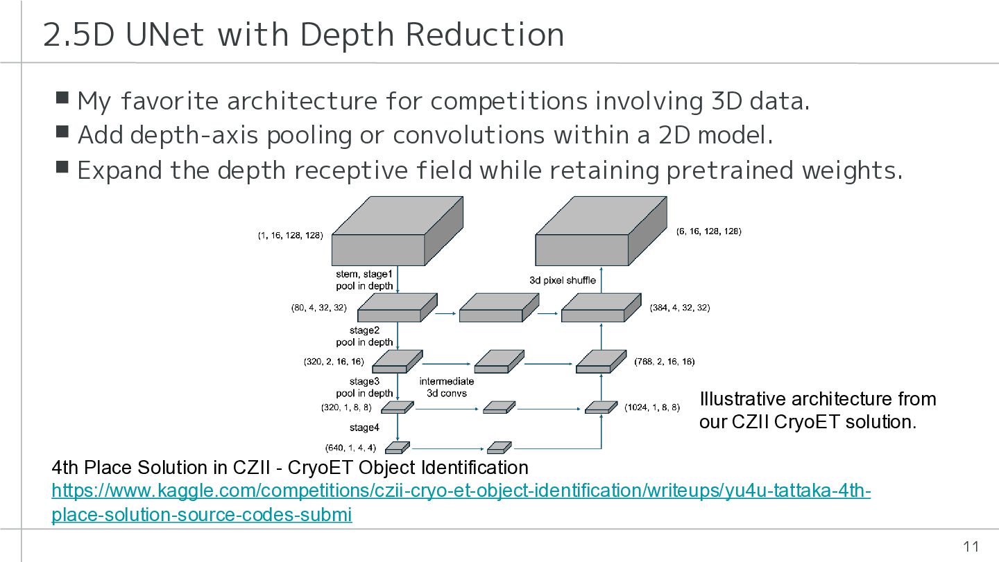
11. 2.5D UNet with Depth Reduction ▪ My favorite architecture for competitions involving 3D data. ▪ Add depth-axis pooling or convolutions within a 2D model. ▪ Expand the depth receptive field while retaining pretrained weights. Illustrative architecture from our CZII CryoET solution. 4th Place Solution in CZII - CryoET Object Identification https://www.kaggle.com/competitions/czii-cryo-et-object-identification/writeups/yu4u-tattaka-4thplace-solution-source-codes-submi 11
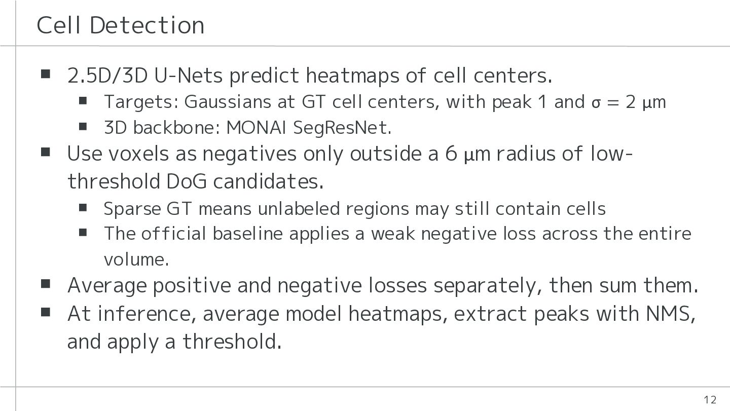
12. Cell Detection ▪ 2.5D/3D U-Nets predict heatmaps of cell centers. ▪ Targets: Gaussians at GT cell centers, with peak 1 and σ = 2 µm ▪ 3D backbone: MONAI SegResNet. ▪ Use voxels as negatives only outside a 6 µm radius of lowthreshold DoG candidates. ▪ Sparse GT means unlabeled regions may still contain cells ▪ The official baseline applies a weak negative loss across the entire volume. ▪ Average positive and negative losses separately, then sum them. ▪ At inference, average model heatmaps, extract peaks with NMS, and apply a threshold. 12
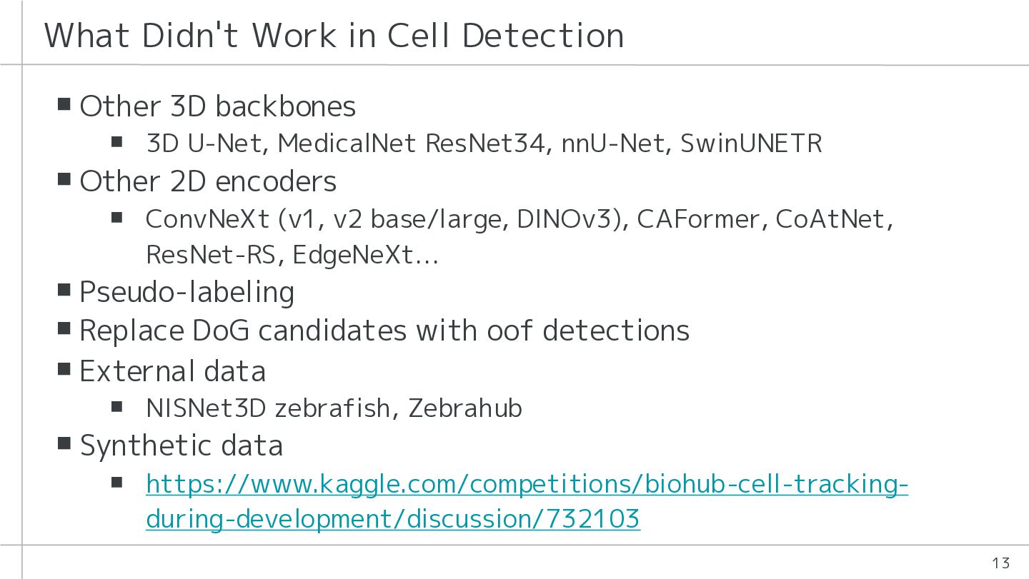
13. What Didn't Work in Cell Detection ▪ Other 3D backbones ▪ 3D U-Net, MedicalNet ResNet34, nnU-Net, SwinUNETR ▪ Other 2D encoders ▪ ConvNeXt (v1, v2 base/large, DINOv3), CAFormer, CoAtNet, ResNet-RS, EdgeNeXt… ▪ Pseudo-labeling ▪ Replace DoG candidates with oof detections ▪ External data ▪ NISNet3D zebrafish, Zebrahub ▪ Synthetic data ▪ https://www.kaggle.com/competitions/biohub-cell-trackingduring-development/discussion/732103 13
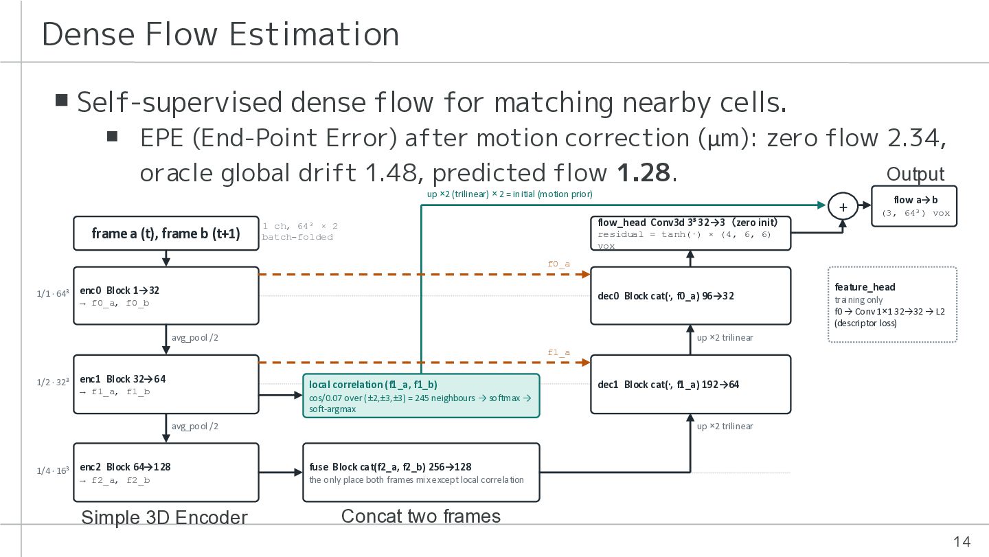
14. Dense Flow Estimation ▪ Self-supervised dense flow for matching nearby cells. ▪ EPE (End-Point Error) after motion correction (µm): zero flow 2.34, oracle global drift 1.48, predicted flow 1.28. Output up ×2 (trilinear) × 2 = initial (motion prior) frame a (t), frame b (t+1) + flow a→b (3, 64³) vox flow_head Conv3d 3³ 32→3（zero init） 1 ch, 64³ × 2 batch-folded residual = tanh(·) × (4, 6, 6) vox f0_a 1/1 · 64³ enc0 Block 1→32 dec0 Block cat(·, f0_a) 96→32 → f0_a, f0_b feature_head training only f0 → Conv 1×1 32→32 → L2 (descriptor loss) up ×2 trilinear avg_pool /2 f1_a 1/2 · 32³ enc1 Block 32→64 local correlation (f1_a, f1_b) → f1_a, f1_b up ×2 trilinear avg_pool /2 1/4 · 16³ dec1 Block cat(·, f1_a) 192→64 cos/0.07 over (±2,±3,±3) = 245 neighbours → softmax → soft-argmax enc2 Block 64→128 fuse Block cat(f2_a, f2_b) 256→128 → f2_a, f2_b the only place both frames mix except local correlation Simple 3D Encoder Concat two frames 14
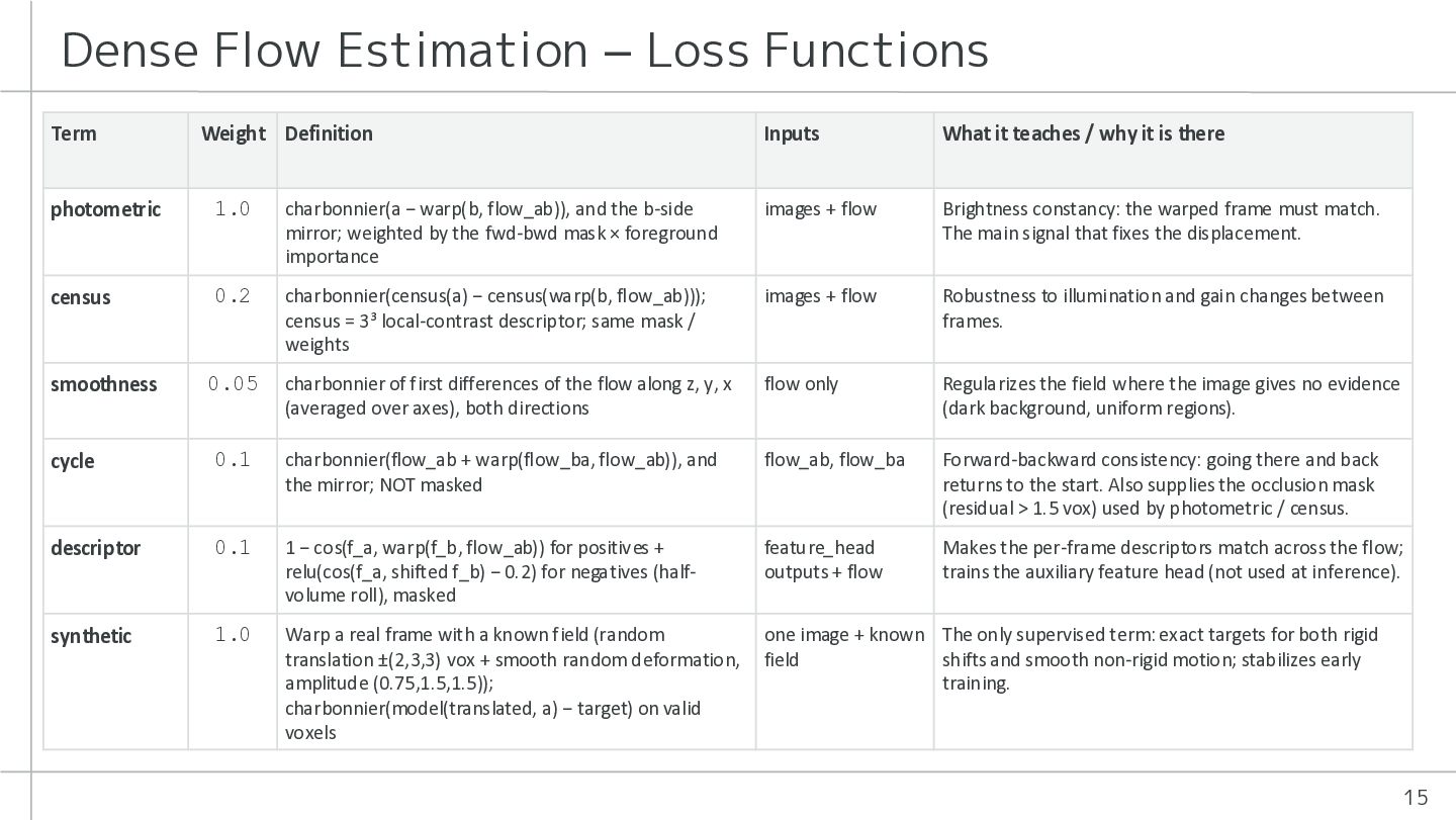
15. Dense Flow Estimation – Loss Functions Term Weight Definition Inputs What it teaches / why it is there photometric 1.0 charbonnier(a − warp(b, flow_ab)), and the b-side mirror; weighted by the fwd-bwd mask × foreground importance images + flow Brightness constancy: the warped frame must match. The main signal that fixes the displacement. census 0.2 charbonnier(census(a) − census(warp(b, flow_ab))); census = 3³ local-contrast descriptor; same mask / weights images + flow Robustness to illumination and gain changes between frames. smoothness 0.05 charbonnier of first differences of the flow along z, y, x (averaged over axes), both directions flow only Regularizes the field where the image gives no evidence (dark background, uniform regions). cycle 0.1 charbonnier(flow_ab + warp(flow_ba, flow_ab)), and the mirror; NOT masked flow_ab, flow_ba Forward-backward consistency: going there and back returns to the start. Also supplies the occlusion mask (residual > 1.5 vox) used by photometric / census. descriptor 0.1 1 − cos(f_a, warp(f_b, flow_ab)) for positives + relu(cos(f_a, shifted f_b) − 0.2) for negatives (halfvolume roll), masked feature_head outputs + flow Makes the per-frame descriptors match across the flow; trains the auxiliary feature head (not used at inference). synthetic 1.0 Warp a real frame with a known field (random translation ±(2,3,3) vox + smooth random deformation, amplitude (0.75,1.5,1.5)); charbonnier(model(translated, a) − target) on valid voxels one image + known The only supervised term: exact targets for both rigid field shifts and smooth non-rigid motion; stabilizes early training. 15
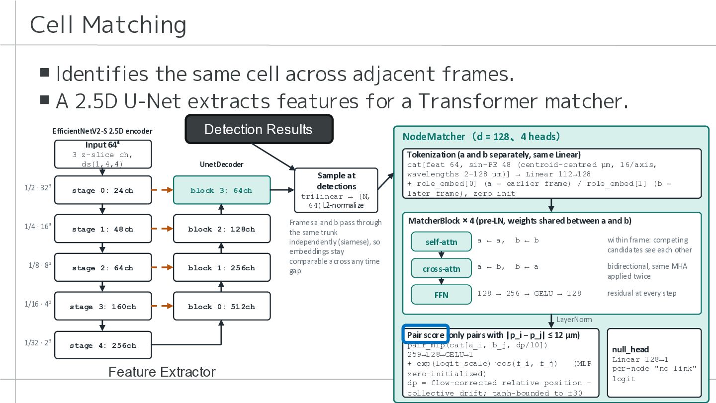
16. Cell Matching ▪ Identifies the same cell across adjacent frames. ▪ A 2.5D U-Net extracts features for a Transformer matcher. EfficientNetV2-S 2.5D encoder Detection Results NodeMatcher（d = 128、4 heads） Input 64³ 3 z-slice ch, ds(1,4,4) Tokenization (a and b separately, same Linear) UnetDecoder 1/2 · 32³ stage 0: 24ch block 3: 64ch 1/4 · 16³ stage 1: 48ch block 2: 128ch 1/8 · 8³ stage 2: 64ch block 1: 256ch 1/16 · 4³ stage 3: 160ch block 0: 512ch Sample at detections trilinear → (N, 64)L2-normalize Frames a and b pass through the same trunk independently (siamese), so embeddings stay comparable across any time gap cat[feat 64, sin-PE 48 (centroid-centred µm, 16/axis, wavelengths 2–128 µm)] → Linear 112→128 + role_embed[0] (a = earlier frame) / role_embed[1] (b = later frame), zero init MatcherBlock × 4 (pre-LN, weights shared between a and b) self-attn a ← a, b ← b within frame: competing candidates see each other cross-attn a ← b, b ← a bidirectional, same MHA applied twice 128 → 256 → GELU → 128 residual at every step FFN LayerNorm 1/32 · 2³ Pair score (only pairs with |p_i − p_j| ≤ 12 µm) stage 4: 256ch Feature Extractor pair_mlp(cat[a_i, b_j, dp/10]) 259→128→GELU→1 + exp(logit_scale)·cos(f_i, f_j) (MLP zero-initialized) dp = flow-corrected relative position − collective drift; tanh-bounded to ±30 null_head Linear 128→1 per-node "no link" logit 16
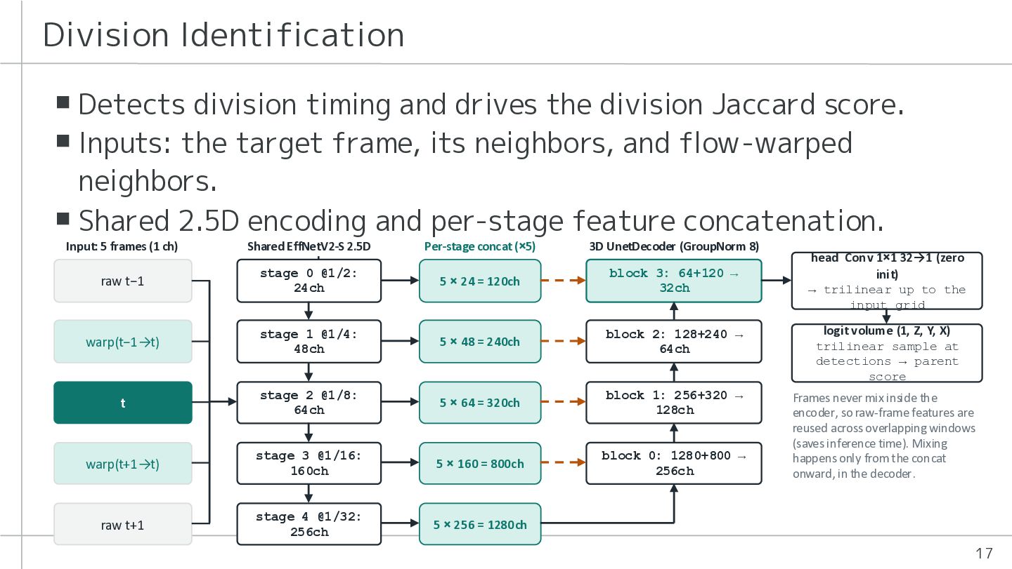
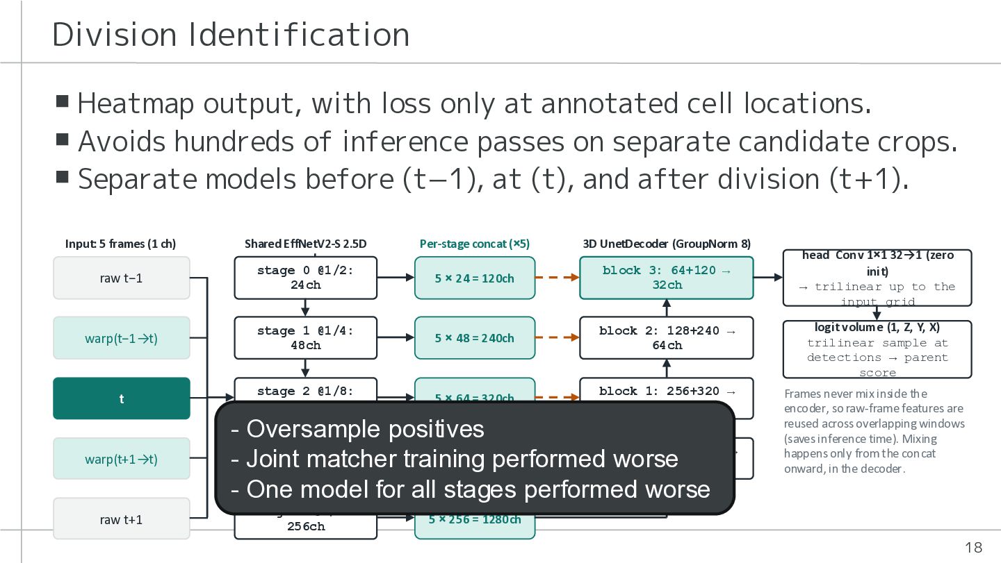
17. Division Identification ▪ Detects division timing and drives the division Jaccard score. ▪ Inputs: the target frame, its neighbors, and flow-warped neighbors. ▪ Shared 2.5D encoding and per-stage feature concatenation. Input: 5 frames (1 ch) raw t−1 Shared EffNetV2-S 2.5D encoder stage 0 @1/2: 24ch Per-stage concat (×5) 3D UnetDecoder (GroupNorm 8) 5 × 24 = 120ch block 3: 64+120 → 32ch warp(t−1→t) stage 1 @1/4: 48ch 5 × 48 = 240ch block 2: 128+240 → 64ch logit volume (1, Z, Y, X) trilinear sample at detections → parent score t stage 2 @1/8: 64ch 5 × 64 = 320ch block 1: 256+320 → 128ch warp(t+1→t) stage 3 @1/16: 160ch 5 × 160 = 800ch block 0: 1280+800 → 256ch Frames never mix inside the encoder, so raw-frame features are reused across overlapping windows (saves inference time). Mixing happens only from the concat onward, in the decoder. raw t+1 stage 4 @1/32: 256ch 5 × 256 = 1280ch head Conv 1×1 32→1 (zero init) → trilinear up to the input grid 17
18. Division Identification ▪ Heatmap output, with loss only at annotated cell locations. ▪ Avoids hundreds of inference passes on separate candidate crops. ▪ Separate models before (t−1), at (t), and after division (t+1). Input: 5 frames (1 ch) raw t−1 Shared EffNetV2-S 2.5D encoder stage 0 @1/2: 24ch warp(t−1→t) stage 1 @1/4: 48ch 5 × 48 = 240ch block 2: 128+240 → 64ch logit volume (1, Z, Y, X) trilinear sample at detections → parent score t stage 2 @1/8: 64ch 5 × 64 = 320ch block 1: 256+320 → 128ch Frames never mix inside the encoder, so raw-frame features are reused across overlapping windows (saves inference time). Mixing happens only from the concat onward, in the decoder. warp(t+1→t) raw t+1 Per-stage concat (×5) 3D UnetDecoder (GroupNorm 8) 5 × 24 = 120ch block 3: 64+120 → 32ch - Oversample positives stage 3 @1/16: 0: 1280+800 → 5 × 160 = 800ch - Joint matcher training performedblock worse 160ch 256ch - One model for all stages performed worse stage 4 @1/32: 256ch head Conv 1×1 32→1 (zero init) → trilinear up to the input grid 5 × 256 = 1280ch 18
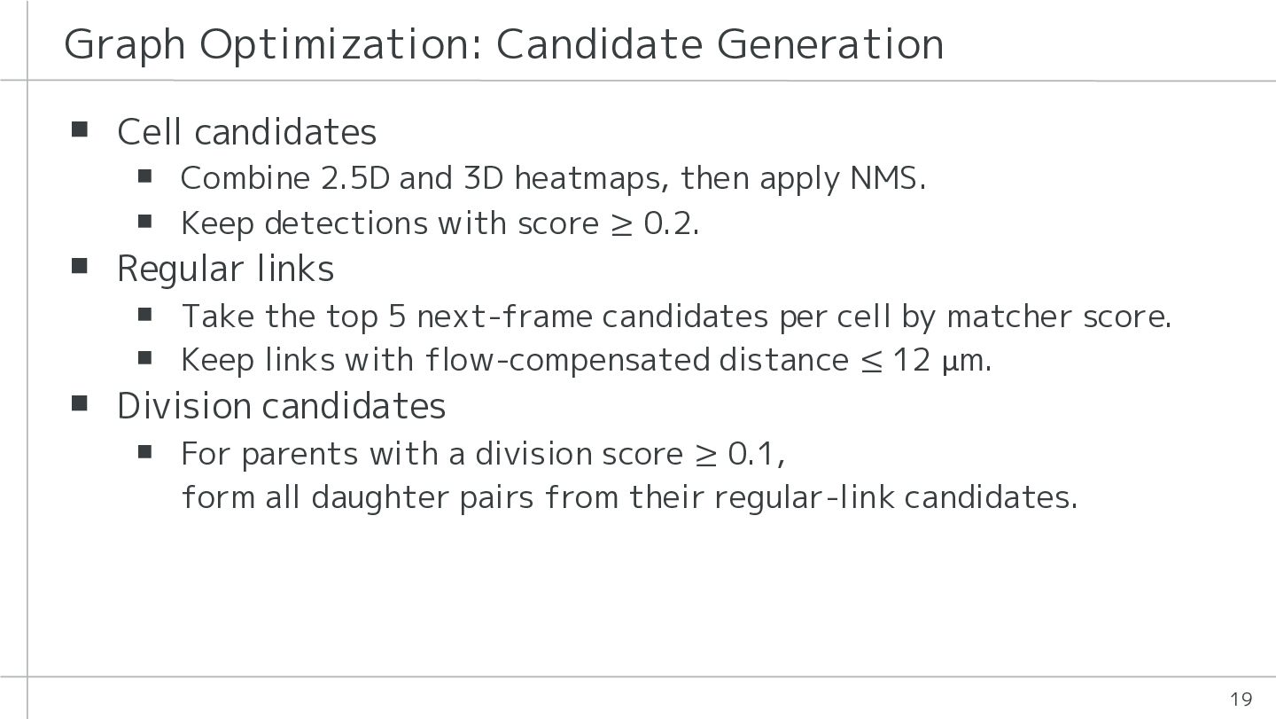
19. Graph Optimization: Candidate Generation ▪ Cell candidates ▪ Combine 2.5D and 3D heatmaps, then apply NMS. ▪ Keep detections with score ≥ 0.2. ▪ Regular links ▪ Take the top 5 next-frame candidates per cell by matcher score. ▪ Keep links with flow-compensated distance ≤ 12 µm. ▪ Division candidates ▪ For parents with a division score ≥ 0.1, form all daughter pairs from their regular-link candidates. 19
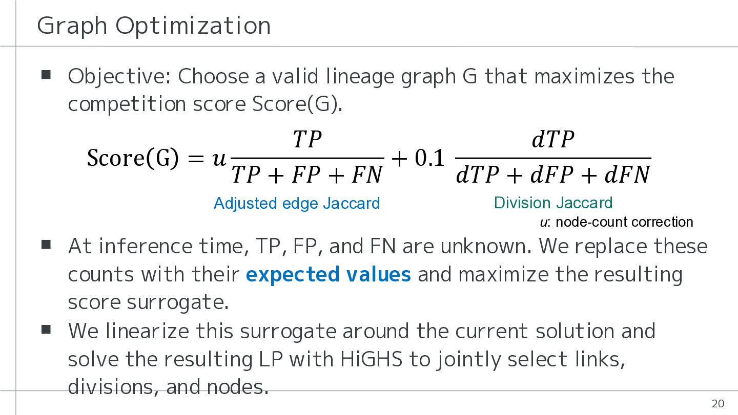
20. Graph Optimization ▪ Objective: Choose a valid lineage graph G that maximizes the competition score Score(G). 𝑇𝑃 𝑑𝑇𝑃 Score G = 𝑢 + 0.1 𝑇𝑃 + 𝐹𝑃 + 𝐹𝑁 𝑑𝑇𝑃 + 𝑑𝐹𝑃 + 𝑑𝐹𝑁 Adjusted edge Jaccard Division Jaccard u: node-count correction ▪ At inference time, TP, FP, and FN are unknown. We replace these counts with their expected values and maximize the resulting score surrogate. ▪ We linearize this surrogate around the current solution and solve the resulting LP with HiGHS to jointly select links, divisions, and nodes. 20
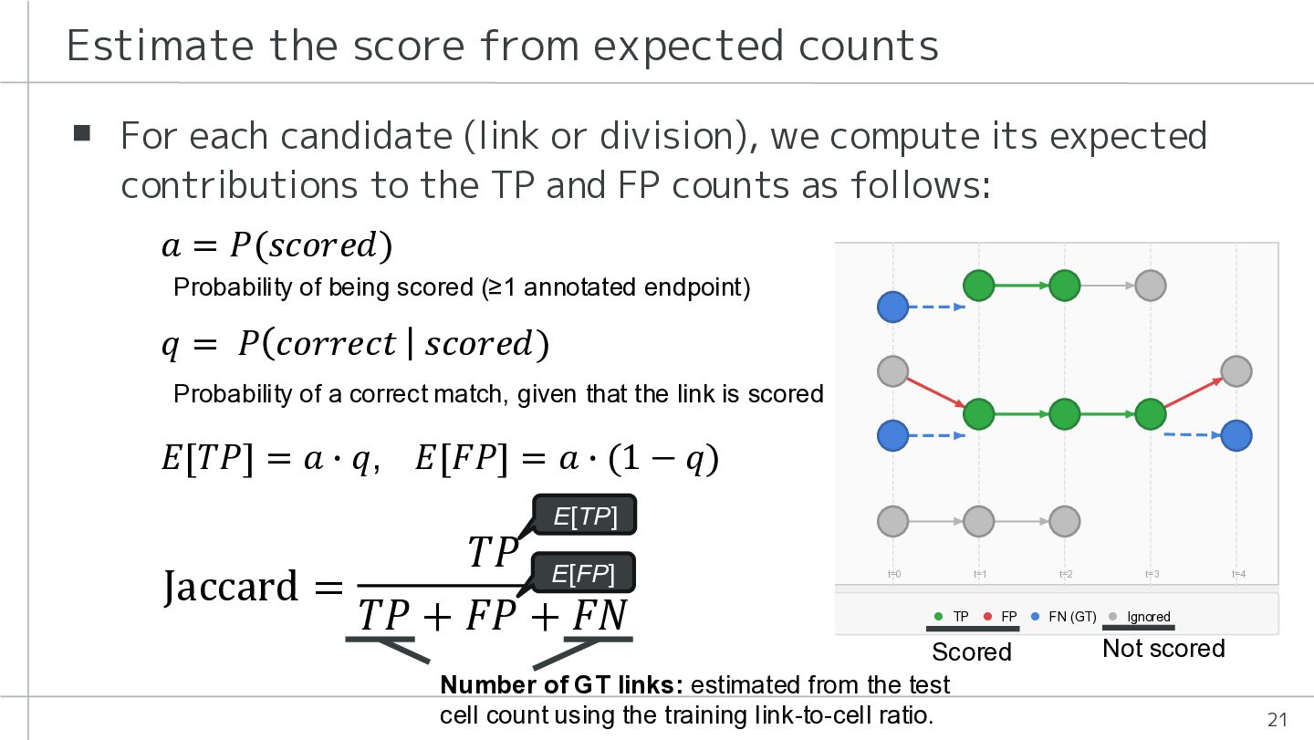
21. Estimate the score from expected counts ▪ For each candidate (link or division), we compute its expected contributions to the TP and FP counts as follows: 𝑎 = 𝑃(𝑠𝑐𝑜𝑟𝑒𝑑) Probability of being scored (≥1 annotated endpoint) 𝑞 = 𝑃 𝑐𝑜𝑟𝑟𝑒𝑐𝑡 𝑠𝑐𝑜𝑟𝑒𝑑) Probability of a correct match, given that the link is scored 𝐸[𝑇𝑃] = 𝑎 ∙ 𝑞, 𝐸[𝐹𝑃] = 𝑎 ∙ (1 − 𝑞) E[TP] 𝑇𝑃 E[FP] Jaccard = 𝑇𝑃 + 𝐹𝑃 + 𝐹𝑁 Scored Number of GT links: estimated from the test cell count using the training link-to-cell ratio. Not scored 21
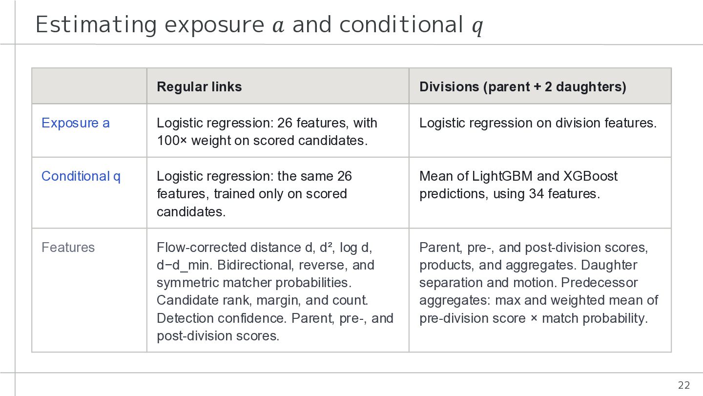
22. Estimating exposure 𝑎 and conditional 𝑞 Regular links Divisions (parent + 2 daughters) Exposure a Logistic regression: 26 features, with 100× weight on scored candidates. Logistic regression on division features. Conditional q Logistic regression: the same 26 features, trained only on scored candidates. Mean of LightGBM and XGBoost predictions, using 34 features. Features Flow-corrected distance d, d², log d, d−d_min. Bidirectional, reverse, and symmetric matcher probabilities. Candidate rank, margin, and count. Detection confidence. Parent, pre-, and post-division scores. Parent, pre-, and post-division scores, products, and aggregates. Daughter separation and motion. Predecessor aggregates: max and weighted mean of pre-division score × match probability. 22
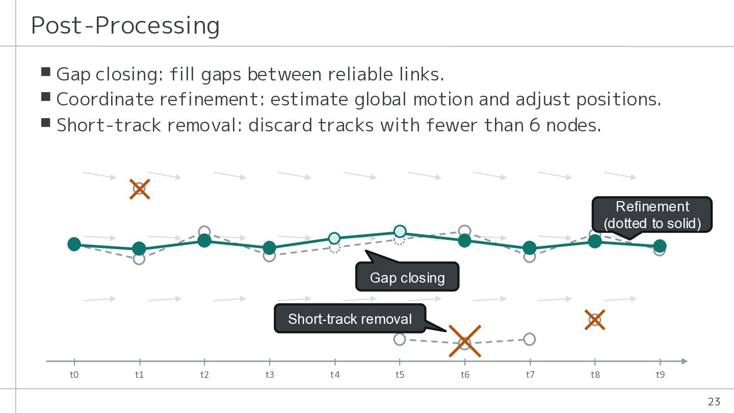
23. Post-Processing ▪ Gap closing: fill gaps between reliable links. ▪ Coordinate refinement: estimate global motion and adjust positions. ▪ Short-track removal: discard tracks with fewer than 6 nodes. Refinement (dotted to solid) Gap closing Short-track removal t0 t1 t2 t3 t4 t5 t6 t7 t8 t9 23
24. Result CV score Public LB Private LB 0.9762 0.978 0.9671 24
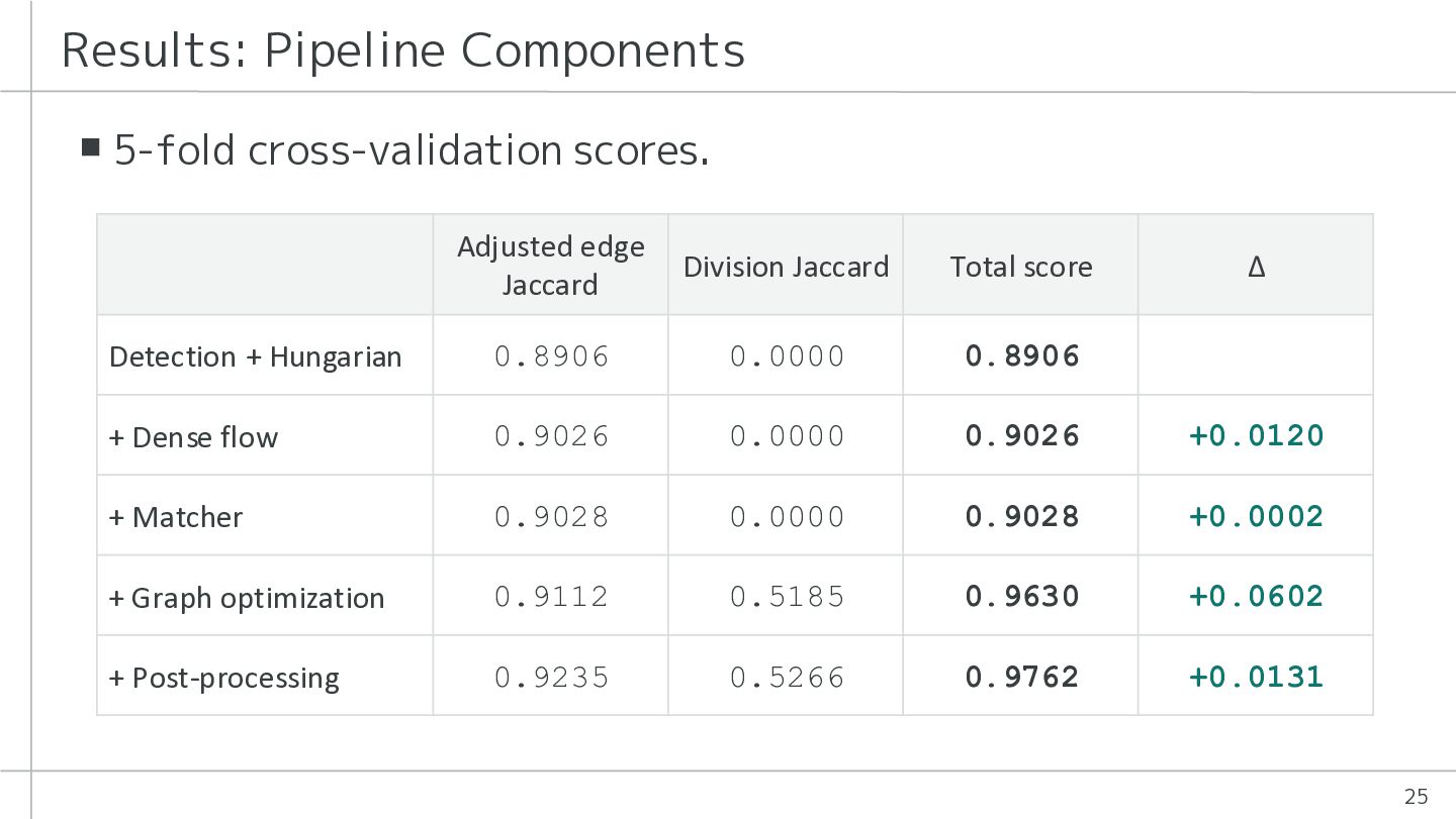
25. Results: Pipeline Components ▪ 5-fold cross-validation scores. Adjusted edge Jaccard Division Jaccard Total score Δ Detection + Hungarian 0.8906 0.0000 0.8906 — + Dense flow 0.9026 0.0000 0.9026 +0.0120 + Matcher 0.9028 0.0000 0.9028 +0.0002 + Graph optimization 0.9112 0.5185 0.9630 +0.0602 + Post-processing 0.9235 0.5266 0.9762 +0.0131 25
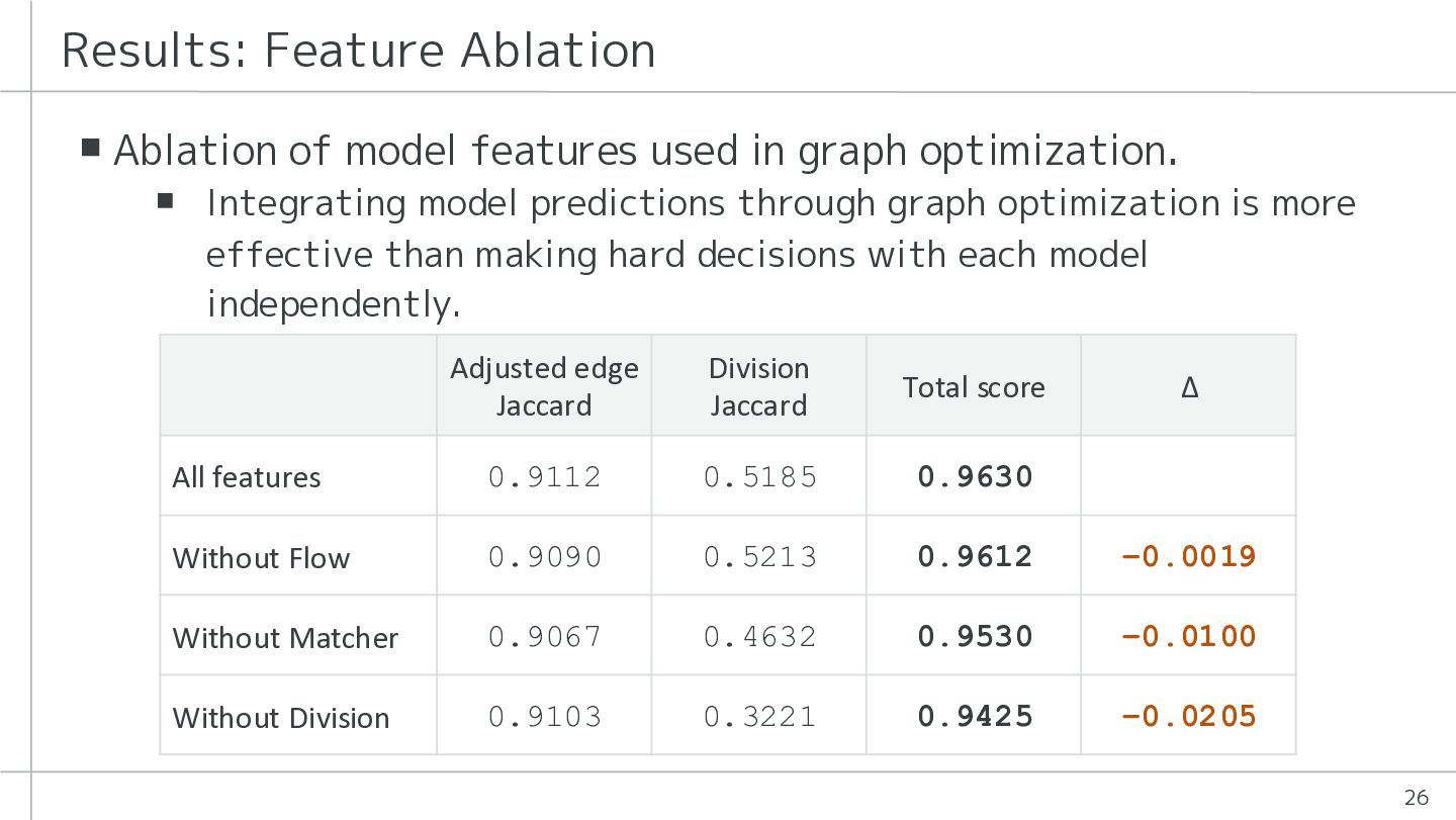
26. Results: Feature Ablation ▪ Ablation of model features used in graph optimization. ▪ Integrating model predictions through graph optimization is more effective than making hard decisions with each model independently. Adjusted edge Jaccard Division Jaccard Total score Δ All features 0.9112 0.5185 0.9630 — Without Flow 0.9090 0.5213 0.9612 −0.0019 Without Matcher 0.9067 0.4632 0.9530 −0.0100 Without Division 0.9103 0.3221 0.9425 −0.0205 26
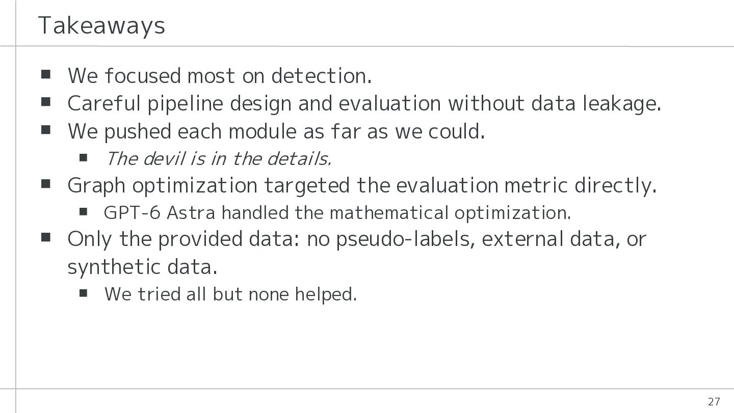
27. Takeaways ▪ We focused most on detection. ▪ Careful pipeline design and evaluation without data leakage. ▪ We pushed each module as far as we could. ▪ The devil is in the details. ▪ Graph optimization targeted the evaluation metric directly. ▪ GPT-6 Astra handled the mathematical optimization. ▪ Only the provided data: no pseudo-labels, external data, or synthetic data. ▪ We tried all but none helped. 27
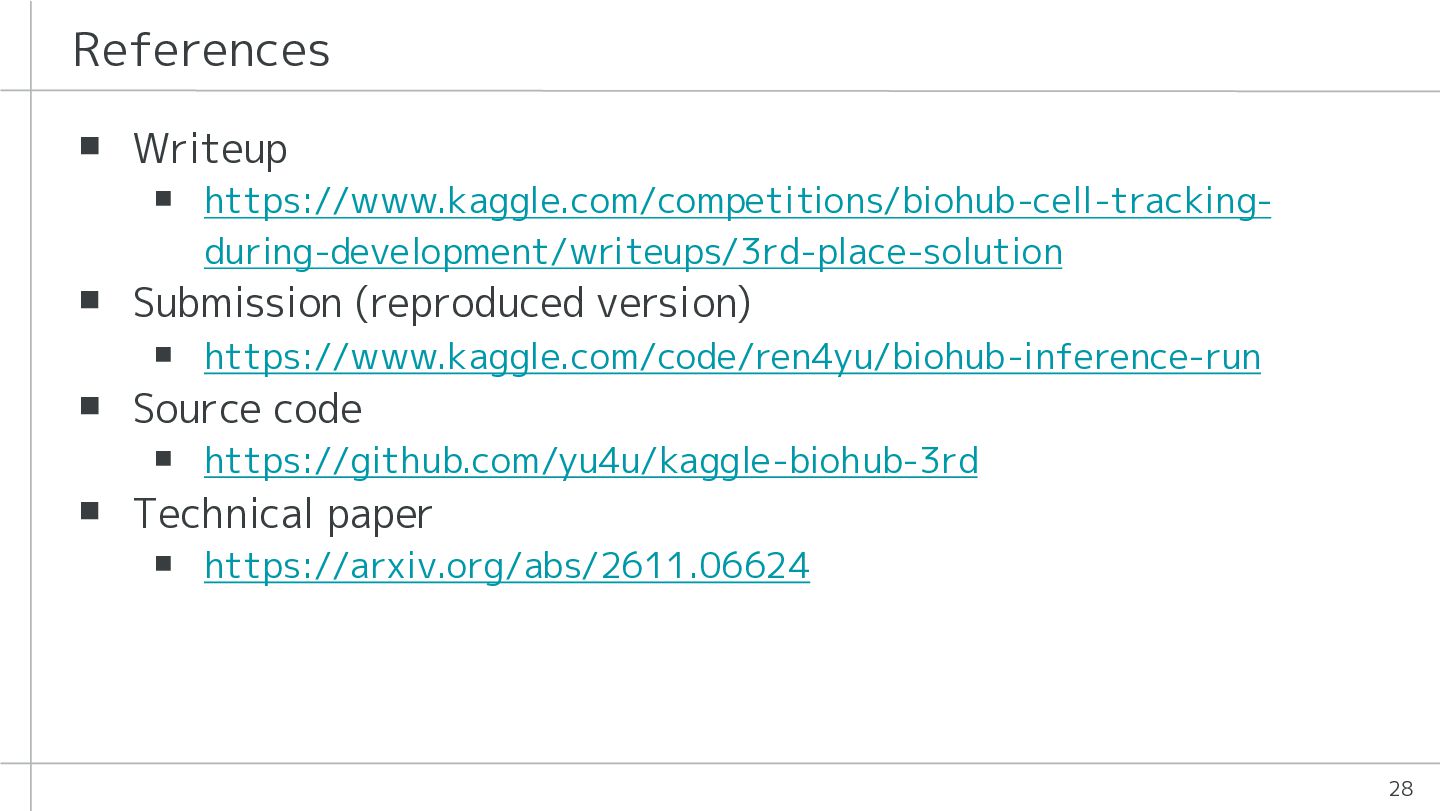
28. References ▪ Writeup ▪ https://www.kaggle.com/competitions/biohub-cell-trackingduring-development/writeups/3rd-place-solution ▪ Submission (reproduced version) ▪ https://www.kaggle.com/code/ren4yu/biohub-inference-run ▪ Source code ▪ https://github.com/yu4u/kaggle-biohub-3rd ▪ Technical paper ▪ https://arxiv.org/abs/2611.06624 28