OSMnxによる街路構造の分析と可視化

2025/02/15 State of the Map Japanでの発表

https://stateofthemap.jp/2024/

Transcript

1. OSMnxによる 街路構造の分析と可視化 Georepublic Japan　大塚 昇 1 2025/02/15 SOTM Japan 2024
2. 使用するコード OSMnxのサンプルコード 2 OSMnxによるコミュニティ分 割のサンプルコード
3. 自己紹介 • 名前 ◦ 大塚昇 • 経歴 ◦ 2010- 不動産関連サービスのWebエンジニア ◦ 2020- 現職にて行政向けアプリのPM ◦ 2020- 社会人博士課程在籍 • 趣味 ◦ 登山、旅行 3
4. 会社紹介 • 合同会社Georepublic Japan • 位置情報系テクノロジー • タスク管理ツールLOBSTA 4
5. 本日の内容 1. Pythonライブラリ「OSMnx」の紹介 2. グラフネットワークのコミュニティ分割とは 3. OSMnxによるコミュニティの可視化 -札幌を事例に- 5
6. Pythonライブラリ「 OSMnx」の紹介 6
7. OSMnxとは • 南カリフォルニア大学のGeoff Boeing教授によって開発され ているPythonライブラリ • NetworkXやGeoPandasと連携 • OpenStreetMapから道路ネットワークを取得できる • 都市の施設、建物の形状、高度データなども取得可能 • 上記の地理空間データを使って、最短経路探索等のネット ワーク分析・可視化ができる 7
8. 道路ネットワークデータの読み込み 8 import osmnx as ox point = (43.07228728953197, 141.3606696070986) # EZOHUB SAPPORO G = ox.graph_from_point(point, dist=300, network_type="drive") fig, ax = ox.plot_graph(G)
9. 建物情報の読み込み 9 point = (43.07228728953197, 141.3606696070986) # EZOHUB SAPPORO tags = {"building": True} gdf = ox.features_from_point(point, dist=300, tags=tags) gdf.shape fig, ax = ox.plot_footprints(gdf, figsize=(3, 3))
10. 合わせ技（ EZOHUB SAPPORO，札幌駅） 10
11. ポイントによる道路ネットワークの読み込み 11 # EZOHUB SAPPOROから１マイルの街路を取得 wurster_hall = (43.07228728953197, 141.3606696070986) one_mile = 1609 # meters G = ox.graph_from_point(wurster_hall, dist=one_mile, network_type="drive") fig, ax = ox.plot_graph(G, node_size=0)
12. ルート検索 12 gdf_nodes, gdf_edges = ox.graph_to_gdfs(G) # 道路の走行距離を追加 G = ox.routing.add_edge_speeds(G) # 道路の所要時間を追加 G = ox.routing.add_edge_travel_times(G) orig = ox.distance.nearest_nodes(G, Y=43.07228728953197, X=141.3606696070986) # EZOHUB SAPPORO dest = ox.distance.nearest_nodes(G, Y=43.06871556428772, X=141.34937048750885) # 札幌駅 # 距離をもとに最短経路を計算 route1 = ox.shortest_path(G, orig, dest, weight="distance") fig, ax = ox.plot_graph_route(G, route1, node_size=0)
13. 距離/所要時間によるルート検索の差異 13 # 距離をもとに最短経路を計算 route1 = ox.shortest_path(G, orig, dest, weight="length") # 所要時間をもとに最短経路を計算 route2 = ox.shortest_path(G, orig, dest, weight="travel_time") # plot the routes fig, ax = ox.plot_graph_routes( G, routes=[route1, route2], route_colors=["r", "y"], route_linewidth=6, node_size=0 )
14. グラフネットワークのコミュニティ分割 14
15. グラフネットワークのコミュニティ分割とは • ネットワーク内で密接に結合したノードのグループを特定する 手法（例：学校のクラス内での友人グループの特定） • Louvain法は、グラフネットワークのコミュニティ分割において 広く使用される効果的なアルゴリズム。ネットワーク内のコミュ ニティ構造の質を評価する指標であるモジュラリティを最大化 する 15
16. ネットワークデータの読み込みと可視化 16 # サンプルグラフの作成 G = nx.karate_club_graph() # 可視化（オプション） pos = nx.spring_layout(G) plt.figure(figsize=(10, 8)) nx.draw(G, pos, node_color='lightblue', node_size=600, with_labels=True, edgecolors='navy', font_color='black', font_weight='bold') plt.show()
17. ネットワークデータのコミュニティ分割 17 import networkx as nx from community import community_louvain # サンプルグラフの作成 G = nx.karate_club_graph() # Fast Unfolding法（Louvain法）の実行 partition = community_louvain.best_partition(G) # 結果の表示 print("ノードとそのコミュニティ :") for node, community_id in partition.items(): print(f"ノード {node}: コミュニティ {community_id}") # コミュニティの数を表示 num_communities = len(set(partition.values())) print(f"\n検出されたコミュニティの数 : {num_communities}") # モジュラリティの計算 modularity = community_louvain.modularity(partition, G) print(f"モジュラリティ : {modularity}"
18. 分割されたコミュニティの可視化 18 pos = nx.spring_layout(G) plt.figure(figsize=(10, 8)) nx.draw(G, pos, node_color=list(partition.values()), cmap=plt.cm.RdYlBu, node_size=600, with_labels=True, edgecolors='navy', font_color='black', font_weight='bold') plt.show()
19. OSMnxによるコミュニティの可視化 - 札幌を事例に - 19
20. 札幌市の道路ネットワークデータの読み込み 20 # 道路ネットワークの取得 place = "Higashi-ku, Sapporo, Hokkaido, Japan" G = ox.graph_from_place(place, network_type="drive") # グラフをGeoDataFrameに変換 nodes, edges = ox.graph_to_gdfs(G) # 地図の作成 fig, ax = plt.subplots(figsize=(15, 15)) # エッジの描画 edges.plot(ax=ax, linewidth=0.5, edgecolor="dimgray") # 背景地図の追加 cx.add_basemap(ax, crs=edges.crs.to_string(), source=cx.providers.OpenStreetMap.Mapnik) # 地図の表示 plt.show()
21. 札幌市のコミュニティ分割の可視化 21 # コミュニティ抽出 communities = community_louvain.best_partition(G_undirected) # コミュニティ情報をノードの属性として追加 nx.set_node_attributes(G, communities, "community") # エッジにコミュニティ情報を追加 for u, v, data in G.edges(data=True): data['community'] = communities[u] # グラフをGeoDataFrameに変換 nodes, edges = ox.graph_to_gdfs(G) # コミュニティごとに色を割り当て unique_communities = set(communities.values()) colors = plt.cm.rainbow(np.linspace(0, 1, len(unique_communities))) color_dict = dict(zip(unique_communities, colors)) # エッジに色を割り当て edges['color'] = edges['community'].map(lambda x: color_dict[x]
22. 利用するデータ • 札幌市のオープンデータ から札幌市の都心部にあ る観光スポット一覧（CSV） を取得 22
23. 札幌市内の主な観光エリア • 札幌駅北界隈 ：下町情緒の繁華街、北海道大学の最寄り駅、東エリアは「第 二のすすきの」と呼ばれる • 札幌駅南・大通界隈 ：商業・業務の中心地、大通公園周辺に高層ビルと多 様な店舗が存在 • 創成川イースト界隈 ：オフィス、マンション、商業施設が混在、歴史的資源あ り • 大通ウェスト界隈 ：歴史的建造物と現代的な街並みが共存 • 狸小路界隈 ：北海道最古の商店街の一つ、約200店舗が軒を連ねる • すすきの界隈 ：日本三大歓楽街の一つ、多様な業種が集積 • 中島公園界隈 ：歴史ある公園、重要文化財の建造物あり、周辺にカフェ多数 23
24. 観光スポットデータの確認 • 札幌駅北界隈 • 札幌駅南・大通界隈 • 狸小路界隈 • すすきの界隈 • 中島公園界隈 • 創成川イースト界隈 • 大通ウェスト界隈 24
25. 観光エリアに変換（バッファ、融合、凸包） • エリアごとにスポットを囲 む凸包を作成し、エリアポ リゴンとして保存 25
26. 道路ネットワークと重ね合わせ • 観光エリアと街路ネット ワークコミュニティを比較し ます 26
27. 札幌駅北界隈 • 創成川通と環状通に囲ま れたエリアまでが札幌駅 北界隈として、おおむね一 かたまりのコミュニティを 形成している 27 環状通 創成川通
28. 創成川イースト界隈 • 大通を境に南北にそれぞ れ別のコミュニティを形成 している 28 大通
29. 札幌駅南・大通界隈 • 駅に近いエリアは創成川 イースト北のコミュニティ に、駅から離れたエリアは すすきの・狸小路のコミュ ニティに属しており、単独 のコミュニティは形成して いない 29
30. 狸小路・すすきの界隈 • 狸小路界隈とすすきの界 隈の街路構造は両者合わ せて一つのコミュニティを 形成している 30
31. 大通ウェスト界隈 • 大通ウェスト界隈は北に 真横に伸びる一つのコミュ ニティ、南に3つのコミュニ ティを形成しており、複雑 な構造となっている 31 大通
32. 中島公園界隈 • 東側では南11条中央線、 札幌環状線を境にコミュニ ティが分割されている 32 南11条中央線 札幌環状線
33. まとめ 33
34. まとめ • OSMnxを使うとOSMの地理空間データを簡単に取得、分析 することができる • グラフネットワークのコミュニティ分割を応用することで、街区 ごとのつながりを把握することができる • 札幌の観光エリアは街路構造としてはさらに小さなコミュニティ を形成していることが確認できた。ただし、狸小路とすすきの は二つの観光エリアが一つのコミュニティを形成していた 34
35. 参考文献 • Geoff Boeing, OSMnx: A Python package to work with graph-theoretic OpenStreetMap street networks, 2017 • GitHub - gboeing/osmnx-examples: Gallery of OSMnx tutorials, usage examples, and feature demonstrations. https://github.com/gboeing/osmnx-examples • Vincent D. Blondel et.al, Fast unfolding of communities in large networks, 2008 35
36. おまけ（１）札幌コミュニティマップ 36
37. おまけ（２）コミュニティ可視化ツール 37
38. おまけ（３）： Isochrone Mapとは • ある地点から一定の時間内に到達可能な範囲を示した地図 • 地理学や都市計画では、ある地点から一定の時間内(例えば 30分以内)に到達可能なエリアを色分けして示した地図 38
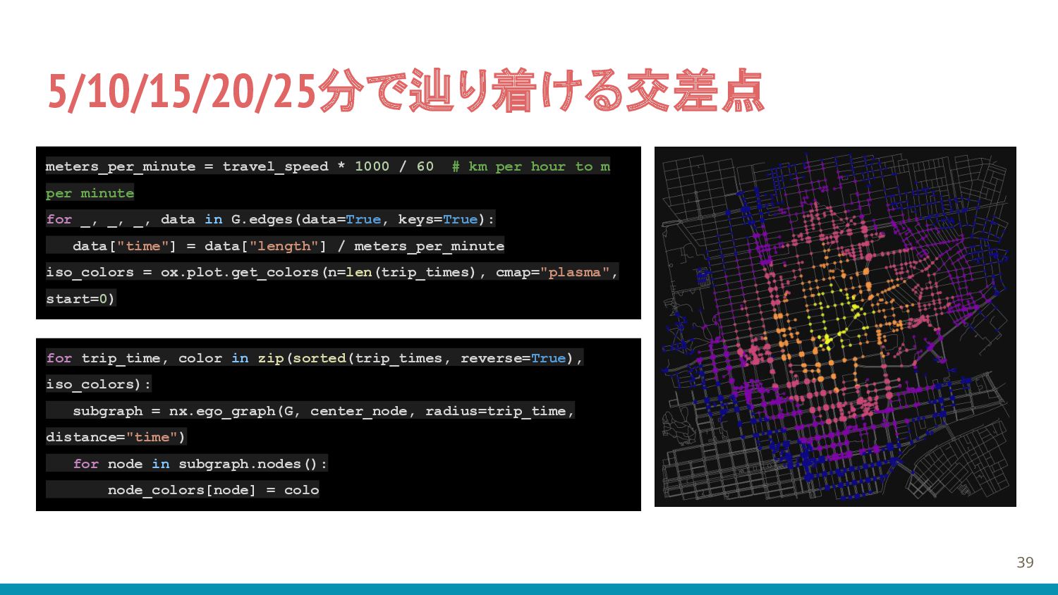
39. 5/10/15/20/25分で辿り着ける交差点 • 39 meters_per_minute = travel_speed * 1000 / 60 # km per hour to m per minute for _, _, _, data in G.edges(data=True, keys=True): data["time"] = data["length"] / meters_per_minute iso_colors = ox.plot.get_colors(n=len(trip_times), cmap="plasma", start=0) for trip_time, color in zip(sorted(trip_times, reverse=True), iso_colors): subgraph = nx.ego_graph(G, center_node, radius=trip_time, distance="time") for node in subgraph.nodes(): node_colors[node] = colo
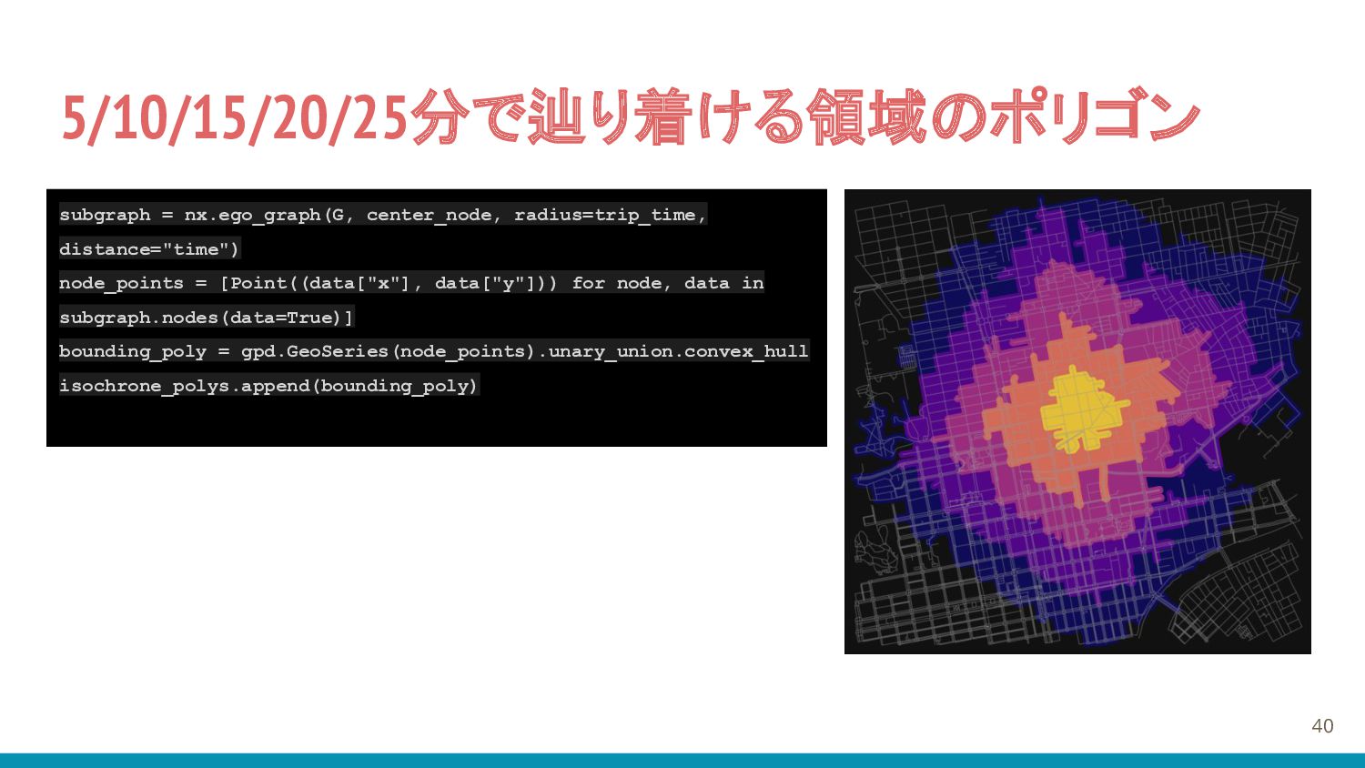
40. 5/10/15/20/25分で辿り着ける領域のポリゴン 40 subgraph = nx.ego_graph(G, center_node, radius=trip_time, distance="time") node_points = [Point((data["x"], data["y"])) for node, data in subgraph.nodes(data=True)] bounding_poly = gpd.GeoSeries(node_points).unary_union.convex_hull isochrone_polys.append(bounding_poly)
41. 背景地図をつけて可視化 41 # グラフをGeoDataFrameに変換 nodes, edges = ox.graph_to_gdfs(G) # 地図の作成 fig, ax = plt.subplots(figsize=(15, 15)) # エッジの描画 edges.plot(ax=ax, linewidth=0.8, edgecolor="dimgray") # Isochroneの描画 gdf.plot(ax=ax, color=iso_colors, ec="none", alpha=0.3, zorder=2) # 背景地図の追加 cx.add_basemap(ax, crs=edges.crs.to_string(), source=cx.providers.OpenStreetMap.Mapnik) # 地図のスタイル調整 ax.set_axis_off() # 地図の表示 plt.show()
42. ご清聴ありがとうございました 42