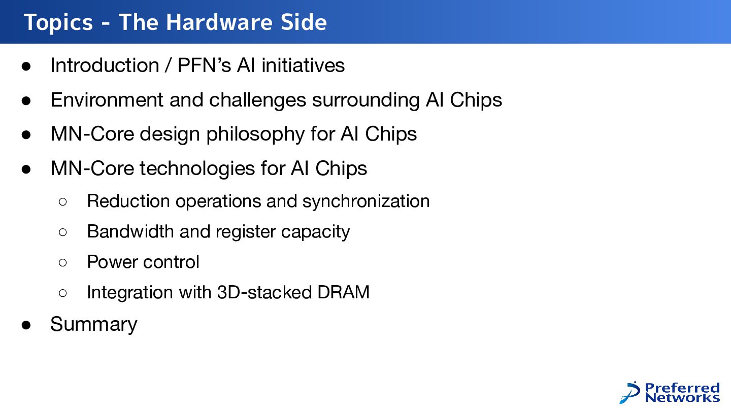
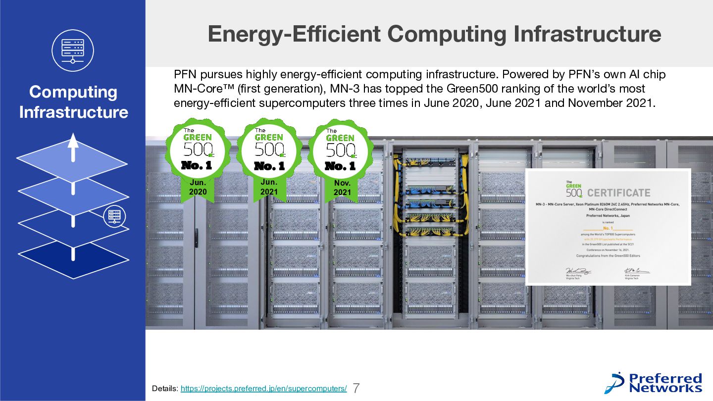
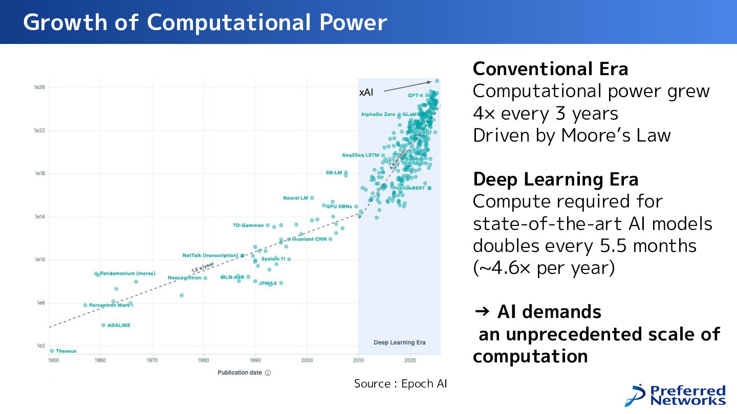
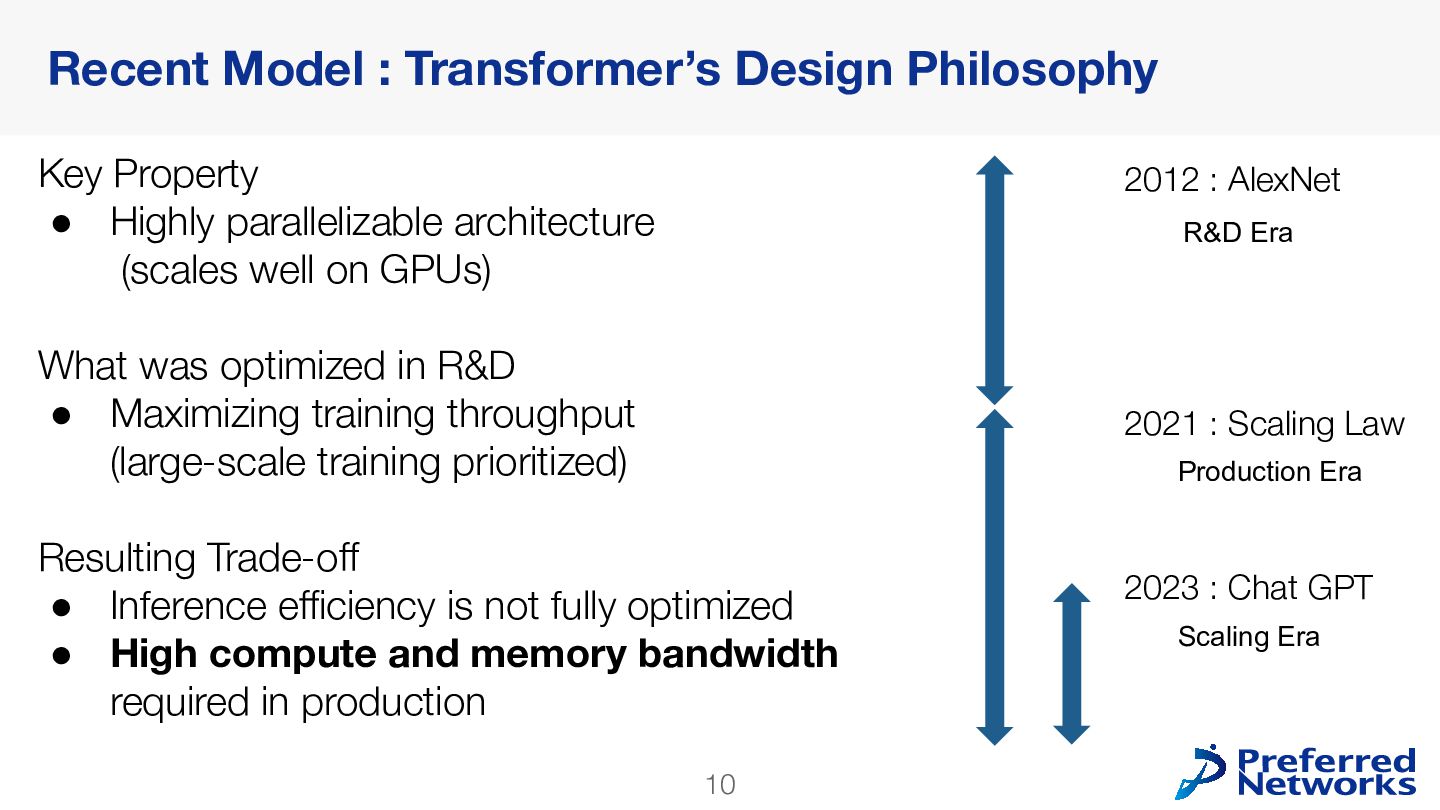
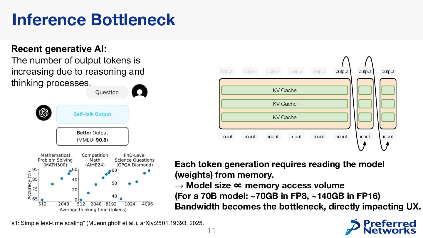
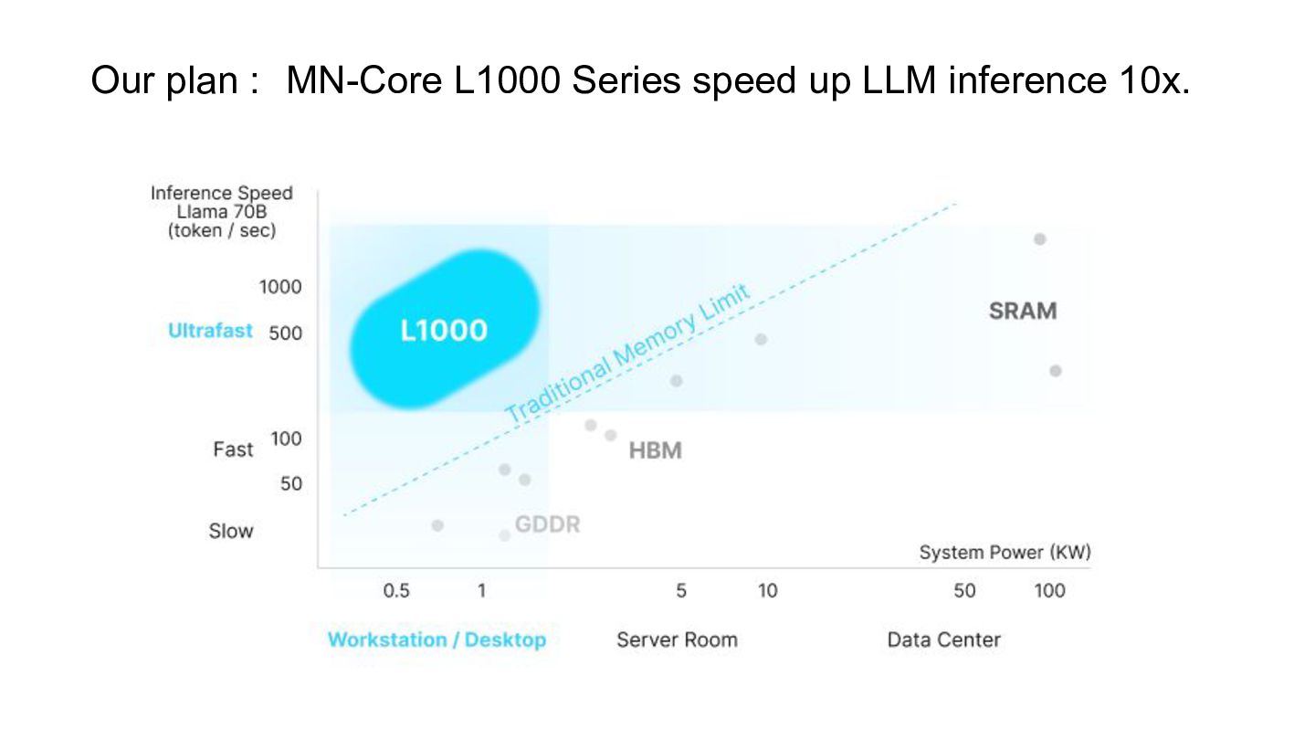
This presentation was for a student discussion session at Kyoto University's Department of Communications and Information Systems, in which Preferred Networks (PFN) introduced the MN-Core series of AI chips from both hardware and software perspectives. It covers the challenges in AI computing such as computing performance, memory bandwidth, and power efficiency; the design philosophy behind MN-Core; and practical aspects of compilers that connect Python to MN-Core, runtime environments, and debugging. | 京都大学 通信情報システム専攻の学生向け談話会の資料です。PFNで開発しているMN-Coreシリーズについて、ハードウェアとソフトウェアの両面から紹介しました。AI計算における計算性能・メモリ帯域・電力効率の課題、それに対するMN-Coreの設計思想、さらにPythonからMN-Coreまでをつなぐコンパイラ・ランタイム・デバッグの実際について説明しています。
![44 from mlsdk import compile def double(input): x = input["x"]](https://files.speakerdeck.com/presentations/f972d7f11ead426cb15298a5640463ef/slide_43.jpg)
![45 from mlsdk import compile def double(input): x = input["x"]](https://files.speakerdeck.com/presentations/f972d7f11ead426cb15298a5640463ef/slide_44.jpg)
![46 from mlsdk import compile def double(input): x = input["x"]](https://files.speakerdeck.com/presentations/f972d7f11ead426cb15298a5640463ef/slide_45.jpg)
![47 Compiler Overview def double(input): x = input["x"] return {"out":](https://files.speakerdeck.com/presentations/f972d7f11ead426cb15298a5640463ef/slide_46.jpg)
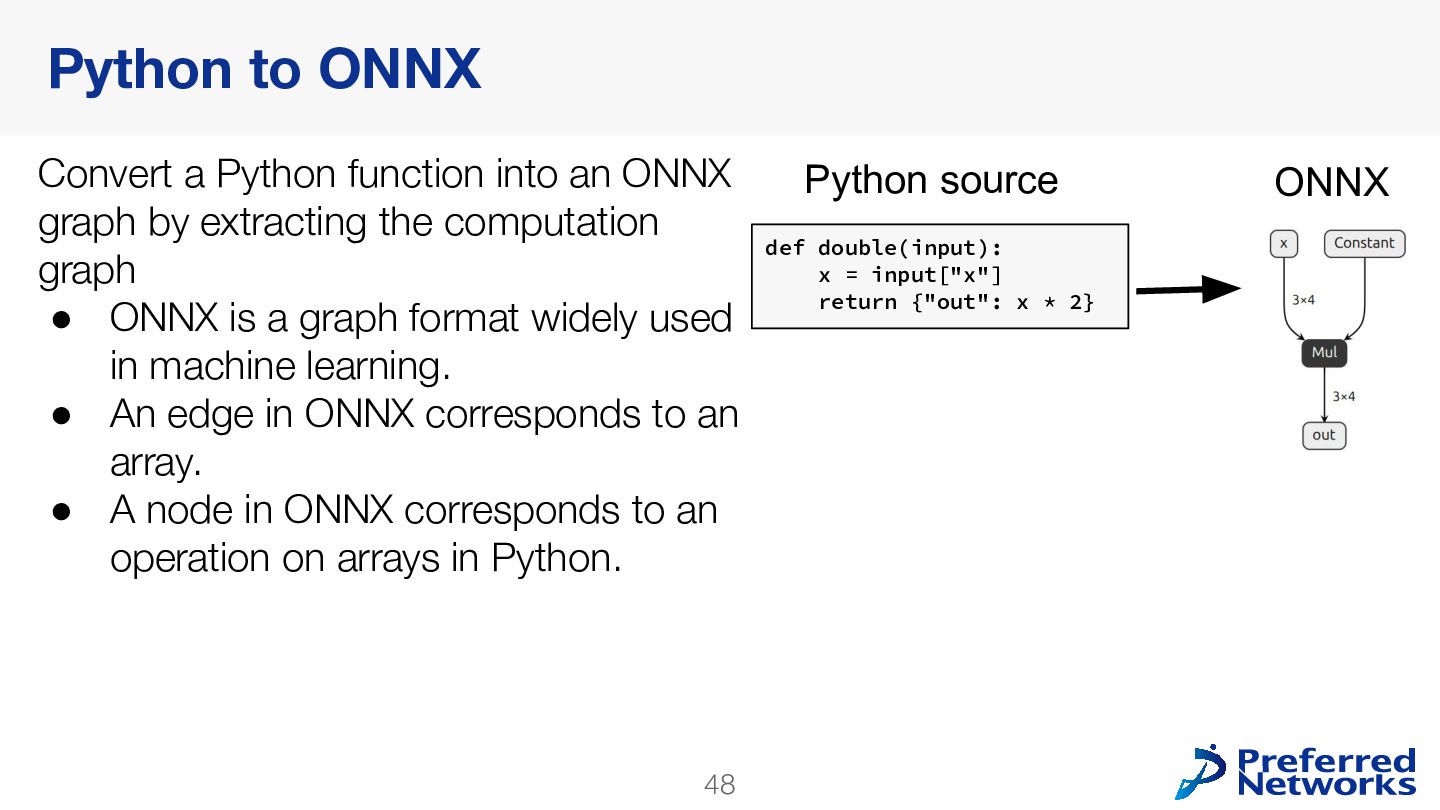
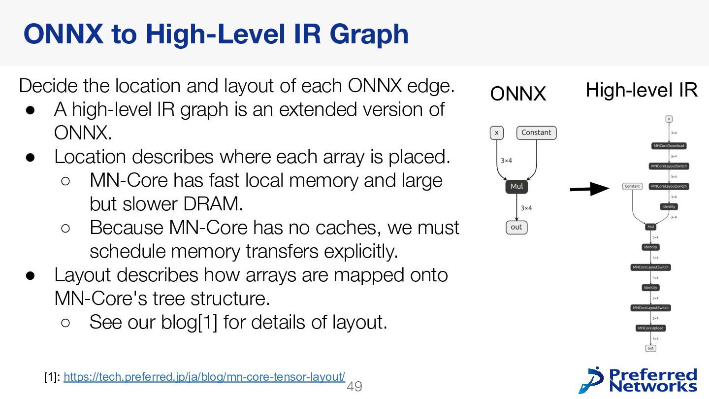
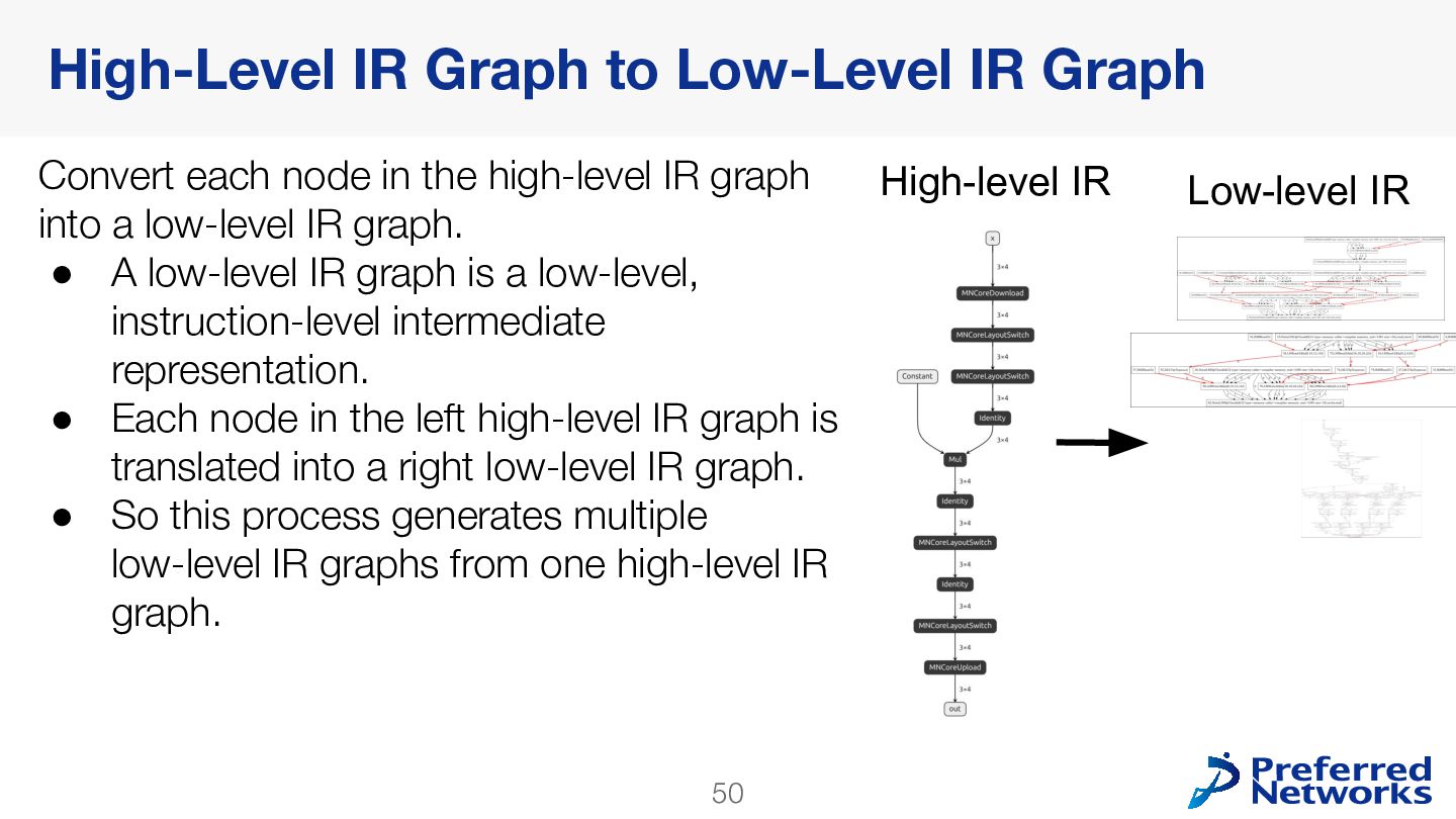
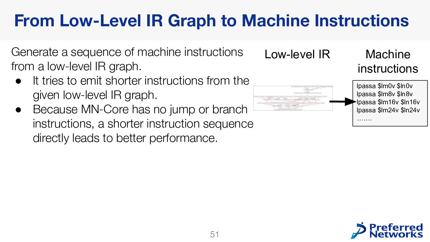
![53 from mlsdk import compile def double(input): x = input["x"]](https://files.speakerdeck.com/presentations/f972d7f11ead426cb15298a5640463ef/slide_52.jpg)