Upgrade to Pro — share decks privately, control downloads, hide ads and more …

DIP_6_Restoration

 DIP_6_Restoration

Avatar for Mohammed Hachama

Mohammed Hachama

September 01, 2025
Tweet

More Decks by Mohammed Hachama

Other Decks in Education

Transcript

  1. Digital Image Processing Restoration (Week 14-15) NHSM - 4th year

    - Fall 2025 - Prof. Mohammed Hachama [email protected] http://hachama.github.io/home/
  2. Outline Introduction Spatial filtering Frequency filtering Morphological filtering Deconvolution NHSM

    - 4th year: Digital Image Processing - Restoration (Week 14-15) - M. Hachama ([email protected]) 2/21
  3. Introduction Image restoration • Improve the visual quality of images

    • Objective methods • Spatial filtering: Low-pass, nonlinear filters, ... • Frequency domain filters • Morphological filtering • Enhancement filters • Inpainting • Subjective methods • Model image degradation • Methods based on degradation NHSM - 4th year: Digital Image Processing - Restoration (Week 14-15) - M. Hachama ([email protected]) 4/21
  4. Introduction Noise and degradation • unwanted distortions that affect the

    quality of an image. NHSM - 4th year: Digital Image Processing - Restoration (Week 14-15) - M. Hachama ([email protected]) 5/21
  5. Introduction Noise • Noise: random variations in pixel intensity values

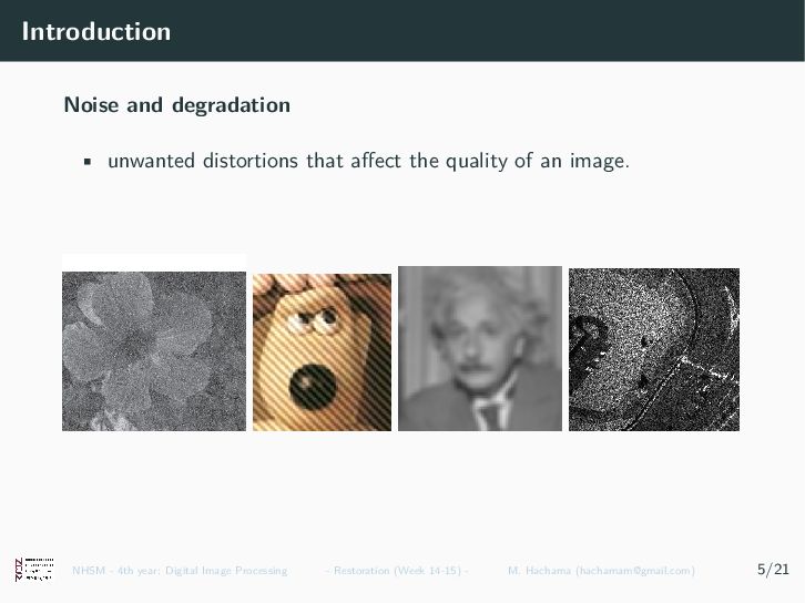
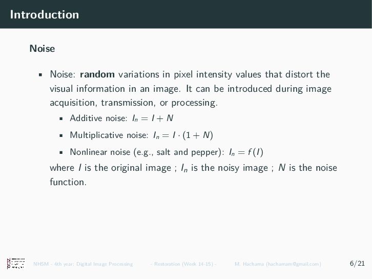
    that distort the visual information in an image. It can be introduced during image acquisition, transmission, or processing. • Additive noise: In = I + N • Multiplicative noise: In = I · (1 + N) • Nonlinear noise (e.g., salt and pepper): In = f (I) where I is the original image ; In is the noisy image ; N is the noise function. NHSM - 4th year: Digital Image Processing - Restoration (Week 14-15) - M. Hachama ([email protected]) 6/21
  6. Introduction Noise estimation • Signal-to-noise ratio (SNR) of a signal

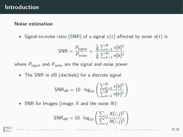
    x(t) affected by noise n(t) is: SNR = Psignal Pnoise = 1 N N k=1 x[k]2 1 N N k=1 n[k]2 where Psignal and Pnoise are the signal and noise power. • The SNR in dB (decibels) for a discrete signal SNRdB = 10 · log10 N k=1 x[k]2 N k=1 n[k]2 • SNR for Images (image X and the noise N): SNRdB = 10 · log10 i,j X(i, j)2 i,j N(i, j)2 NHSM - 4th year: Digital Image Processing - Restoration (Week 14-15) - M. Hachama ([email protected]) 6/21
  7. Introduction Noise estimation • Peak Signal-to-Noise Ratio (PSNR) = Mean

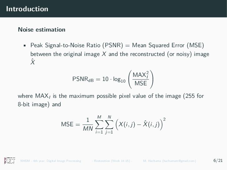
    Squared Error (MSE) between the original image X and the reconstructed (or noisy) image ˆ X PSNRdB = 10 · log10 MAX2 I MSE where MAXI is the maximum possible pixel value of the image (255 for 8-bit image) and MSE = 1 MN M i=1 N j=1 X(i, j) − ˆ X(i, j) 2 NHSM - 4th year: Digital Image Processing - Restoration (Week 14-15) - M. Hachama ([email protected]) 6/21
  8. Introduction Degradation • Degradation = any process that reduces the

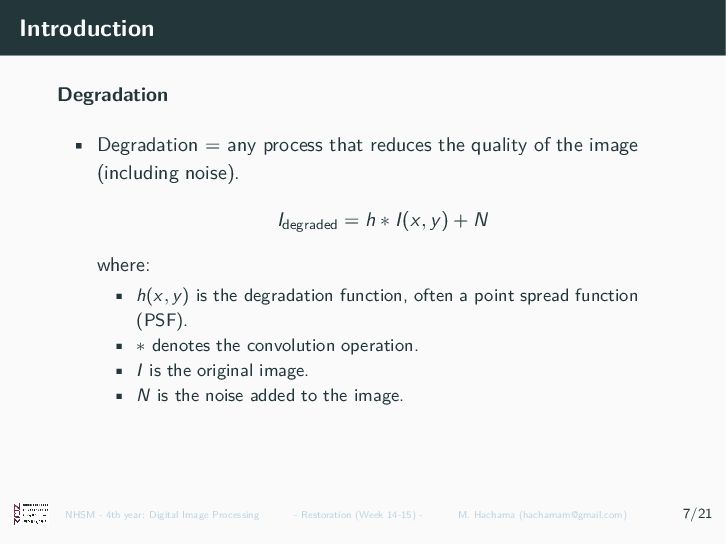
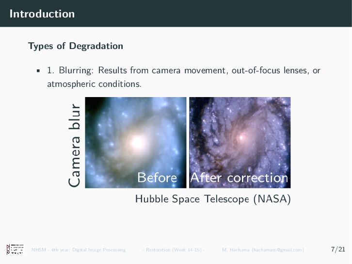
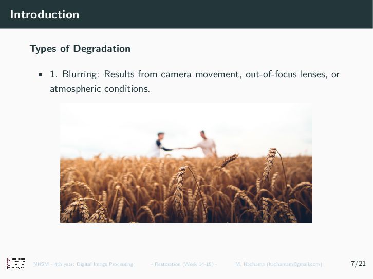
    quality of the image (including noise). Idegraded = h ∗ I(x, y) + N where: • h(x, y) is the degradation function, often a point spread function (PSF). • ∗ denotes the convolution operation. • I is the original image. • N is the noise added to the image. NHSM - 4th year: Digital Image Processing - Restoration (Week 14-15) - M. Hachama ([email protected]) 7/21
  9. Introduction Types of Degradation • 1. Blurring: Results from camera

    movement, out-of-focus lenses, or atmospheric conditions. NHSM - 4th year: Digital Image Processing - Restoration (Week 14-15) - M. Hachama ([email protected]) 7/21
  10. Introduction Types of Degradation • 1. Blurring: Results from camera

    movement, out-of-focus lenses, or atmospheric conditions. NHSM - 4th year: Digital Image Processing - Restoration (Week 14-15) - M. Hachama ([email protected]) 7/21
  11. Introduction Types of Degradation • 1. Blurring: Results from camera

    movement, out-of-focus lenses, or atmospheric conditions. NHSM - 4th year: Digital Image Processing - Restoration (Week 14-15) - M. Hachama ([email protected]) 7/21
  12. Introduction Types of Degradation • 2. Compression leads to misrepresentations

    and artifacts. NHSM - 4th year: Digital Image Processing - Restoration (Week 14-15) - M. Hachama ([email protected]) 7/21
  13. Introduction Types of Degradation • 3.Calibration of the device •

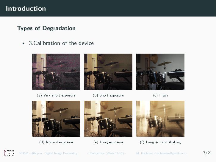
    e.g., Exposure = the amount of light that reaches the camera’s sensor while taking a photo (fractions of a second or entire hours). NHSM - 4th year: Digital Image Processing - Restoration (Week 14-15) - M. Hachama ([email protected]) 7/21
  14. Introduction Types of Degradation • 3.Calibration of the device NHSM

    - 4th year: Digital Image Processing - Restoration (Week 14-15) - M. Hachama ([email protected]) 7/21
  15. Spatial filtering Spatial filtering • Use of masks • Low-pass

    filter: reduces noise but also diminishes image details (more pronounced blur). • High-pass filter: enhances edges and details but amplifies noise. • Band-pass filter: eliminates certain unwanted frequencies. NHSM - 4th year: Digital Image Processing - Restoration (Week 14-15) - M. Hachama ([email protected]) 9/21
  16. Spatial filtering Filters Properties • Separable Filtres NHSM - 4th

    year: Digital Image Processing - Restoration (Week 14-15) - M. Hachama ([email protected]) 9/21
  17. Spatial filtering What is smoothing? • Images are not smooth

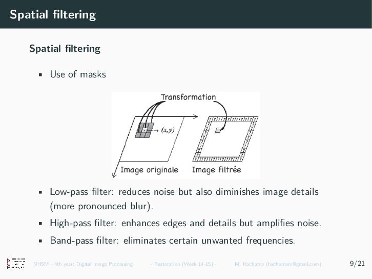
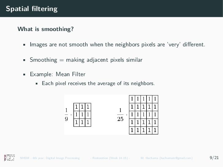
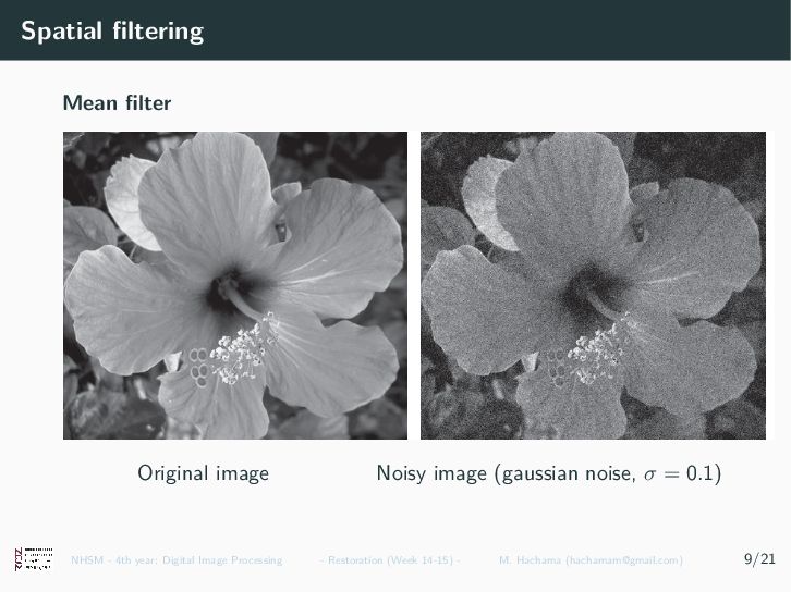
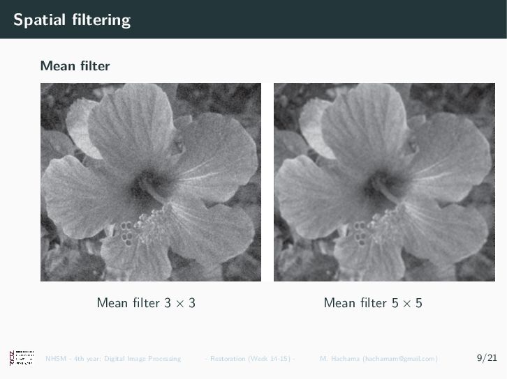
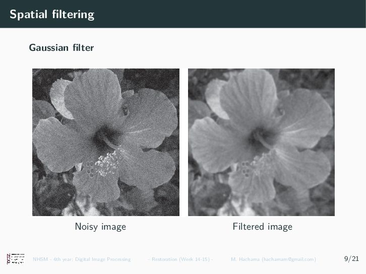
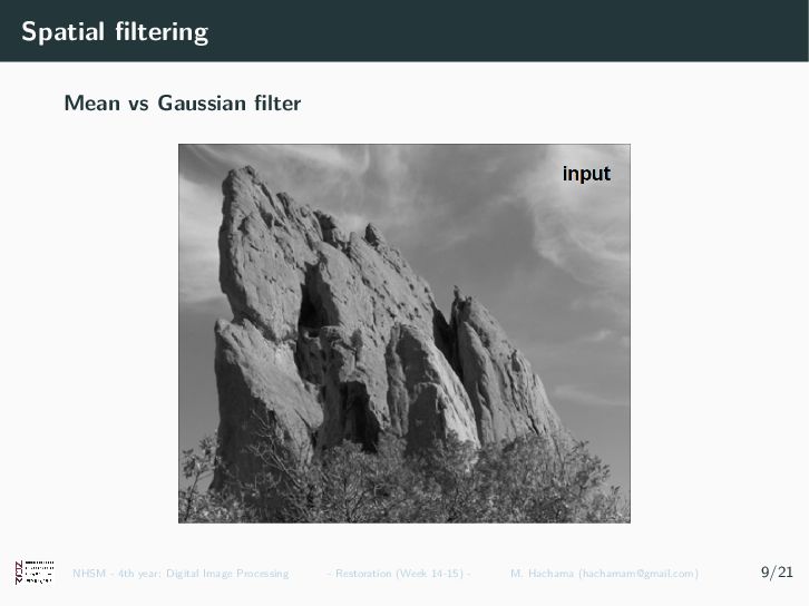
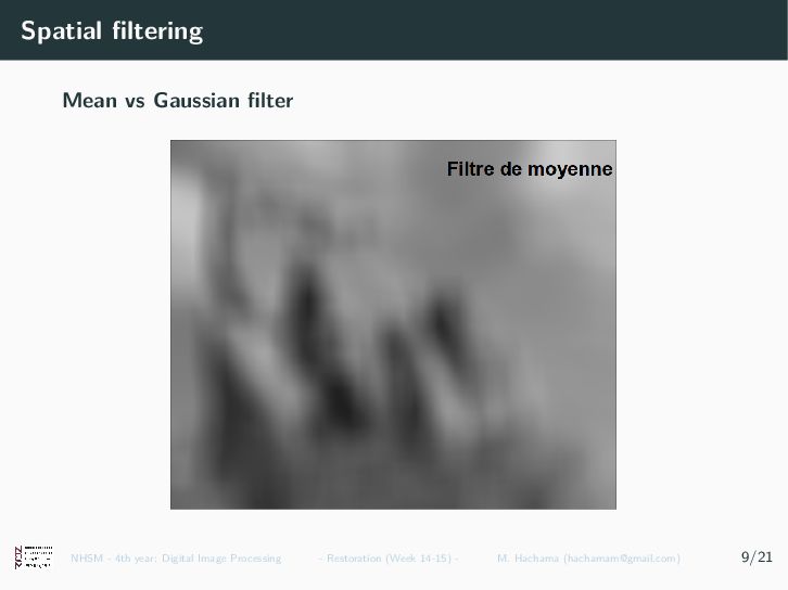
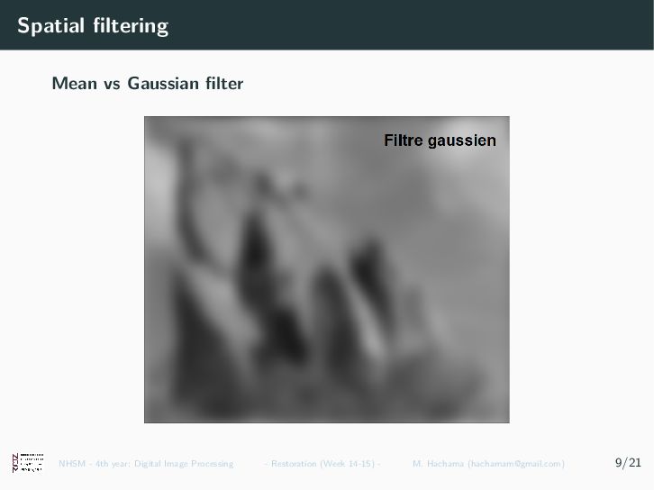
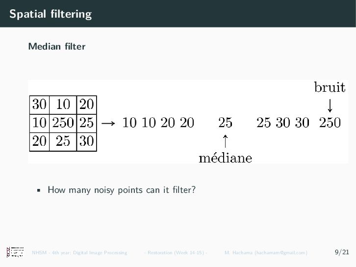
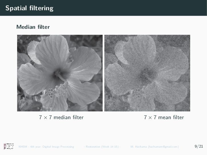
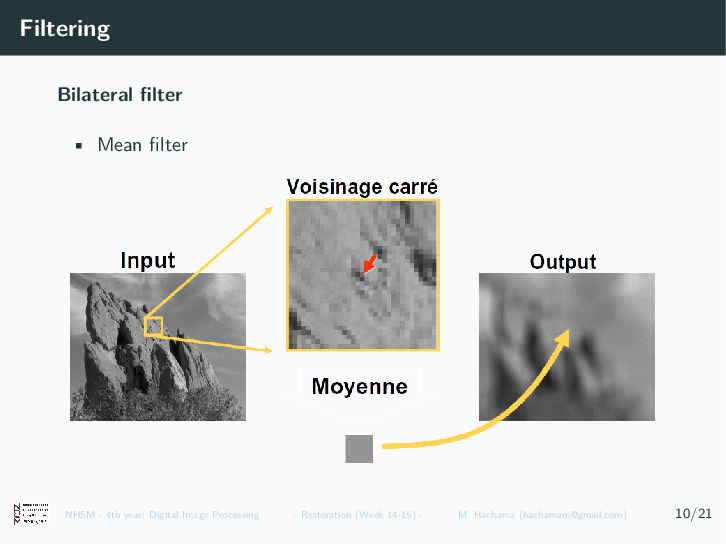
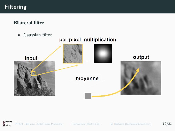
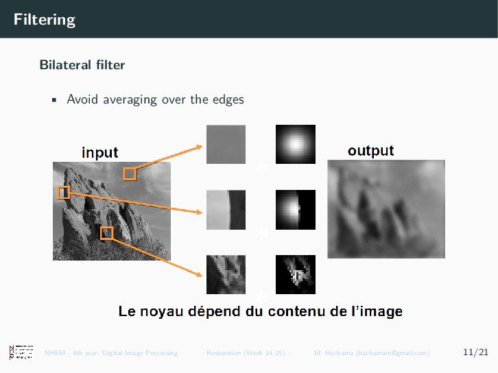
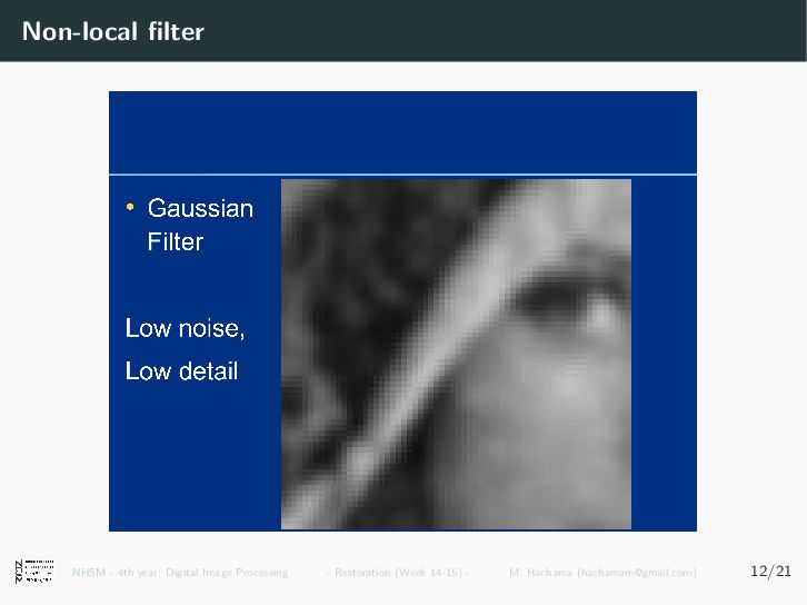
    when the neighbors pixels are ’very’ different. • Smoothing = making adjacent pixels similar • Example: Mean Filter • Each pixel receives the average of its neighbors. NHSM - 4th year: Digital Image Processing - Restoration (Week 14-15) - M. Hachama ([email protected]) 9/21
  18. Spatial filtering Mean filter Original image Noisy image (gaussian noise,

    σ = 0.1) NHSM - 4th year: Digital Image Processing - Restoration (Week 14-15) - M. Hachama ([email protected]) 9/21
  19. Spatial filtering Mean filter Mean filter 3 × 3 Mean

    filter 5 × 5 NHSM - 4th year: Digital Image Processing - Restoration (Week 14-15) - M. Hachama ([email protected]) 9/21
  20. Spatial filtering Gaussian filter (σ = 0.8) NHSM - 4th

    year: Digital Image Processing - Restoration (Week 14-15) - M. Hachama ([email protected]) 9/21
  21. Spatial filtering Gaussian filter Noisy image Filtered image NHSM -

    4th year: Digital Image Processing - Restoration (Week 14-15) - M. Hachama ([email protected]) 9/21
  22. Spatial filtering Mean vs Gaussian filter NHSM - 4th year:

    Digital Image Processing - Restoration (Week 14-15) - M. Hachama ([email protected]) 9/21
  23. Spatial filtering Mean vs Gaussian filter NHSM - 4th year:

    Digital Image Processing - Restoration (Week 14-15) - M. Hachama ([email protected]) 9/21
  24. Spatial filtering Mean vs Gaussian filter NHSM - 4th year:

    Digital Image Processing - Restoration (Week 14-15) - M. Hachama ([email protected]) 9/21
  25. Spatial filtering Median filter • How many noisy points can

    it filter? NHSM - 4th year: Digital Image Processing - Restoration (Week 14-15) - M. Hachama ([email protected]) 9/21
  26. Spatial filtering Median filter Original image Noisy image NHSM -

    4th year: Digital Image Processing - Restoration (Week 14-15) - M. Hachama ([email protected]) 9/21
  27. Spatial filtering Median filter 3 × 3 median filter 3

    × 3 mean filter NHSM - 4th year: Digital Image Processing - Restoration (Week 14-15) - M. Hachama ([email protected]) 9/21
  28. Spatial filtering Median filter 5 × 5 median filter 5

    × 5 mean filter NHSM - 4th year: Digital Image Processing - Restoration (Week 14-15) - M. Hachama ([email protected]) 9/21
  29. Spatial filtering Median filter 7 × 7 median filter 7

    × 7 mean filter NHSM - 4th year: Digital Image Processing - Restoration (Week 14-15) - M. Hachama ([email protected]) 9/21
  30. Filtering Bilateral filter • Mean filter NHSM - 4th year:

    Digital Image Processing - Restoration (Week 14-15) - M. Hachama ([email protected]) 10/21
  31. Filtering Bilateral filter • Gaussian filter NHSM - 4th year:

    Digital Image Processing - Restoration (Week 14-15) - M. Hachama ([email protected]) 10/21
  32. Filtering Bilateral filter • Gaussian filter NHSM - 4th year:

    Digital Image Processing - Restoration (Week 14-15) - M. Hachama ([email protected]) 11/21
  33. Filtering Bilateral filter • Avoid averaging over the edges NHSM

    - 4th year: Digital Image Processing - Restoration (Week 14-15) - M. Hachama ([email protected]) 11/21
  34. Filtering Bilateral filter • Bilateral filter • Adaptive weights NHSM

    - 4th year: Digital Image Processing - Restoration (Week 14-15) - M. Hachama ([email protected]) 11/21
  35. Filtering Bilateral filter • Staircase effect NHSM - 4th year:

    Digital Image Processing - Restoration (Week 14-15) - M. Hachama ([email protected]) 11/21
  36. Filtering Bilateral filter • Texture suppression NHSM - 4th year:

    Digital Image Processing - Restoration (Week 14-15) - M. Hachama ([email protected]) 11/21
  37. Filtering Bilateral filter • Cartoon effect NHSM - 4th year:

    Digital Image Processing - Restoration (Week 14-15) - M. Hachama ([email protected]) 11/21
  38. Filtering Bilateral filter • Cartoon effect NHSM - 4th year:

    Digital Image Processing - Restoration (Week 14-15) - M. Hachama ([email protected]) 11/21
  39. Non-local filter • Like the bilateral filter: averaging ”similar” pixels

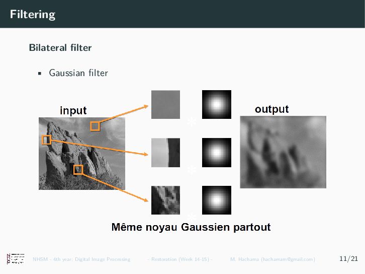
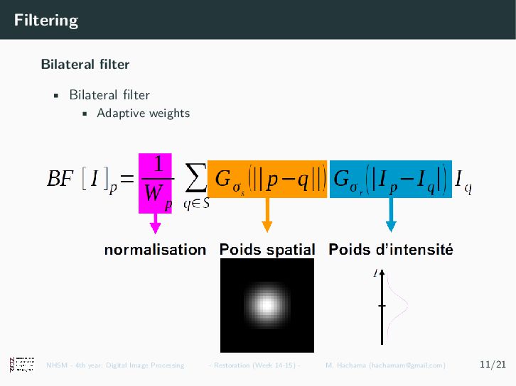
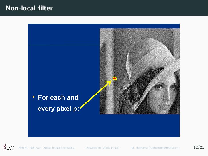
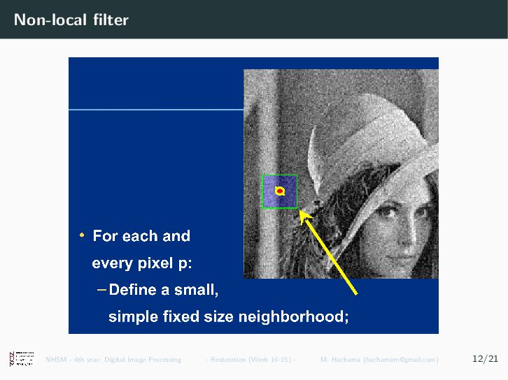
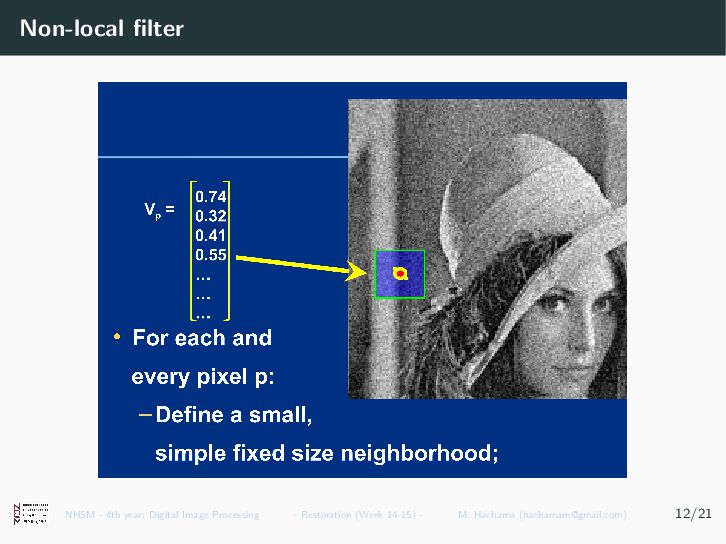
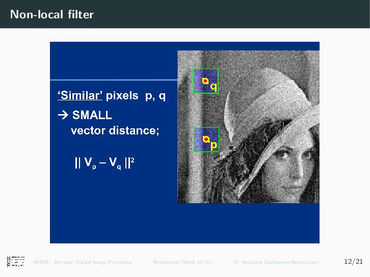
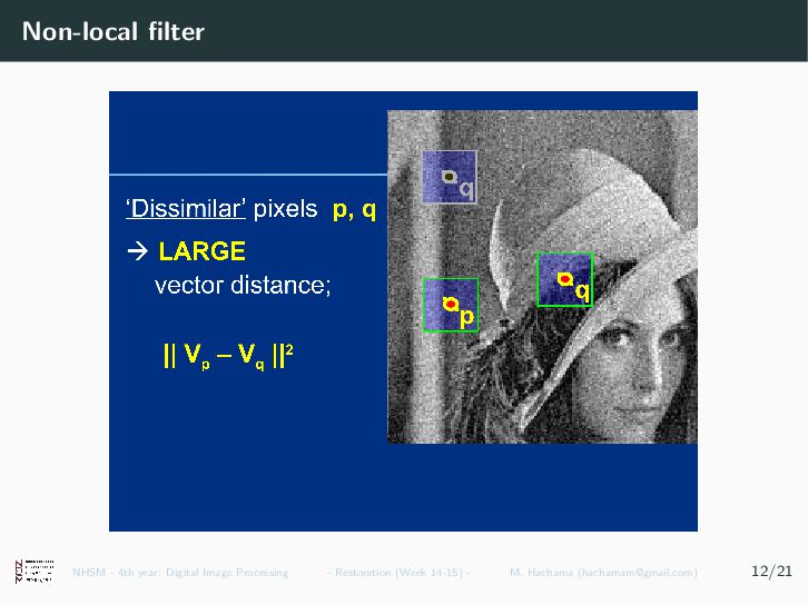
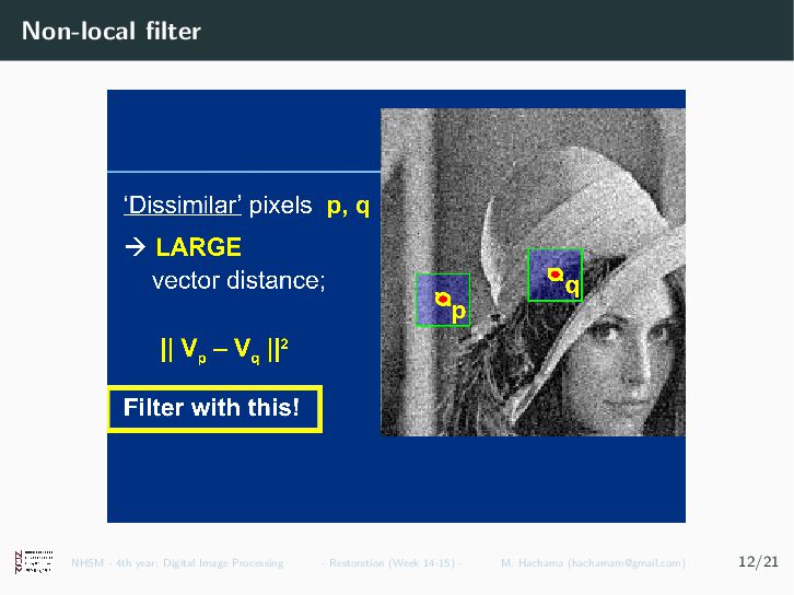
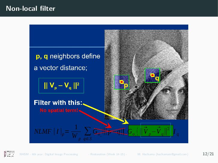
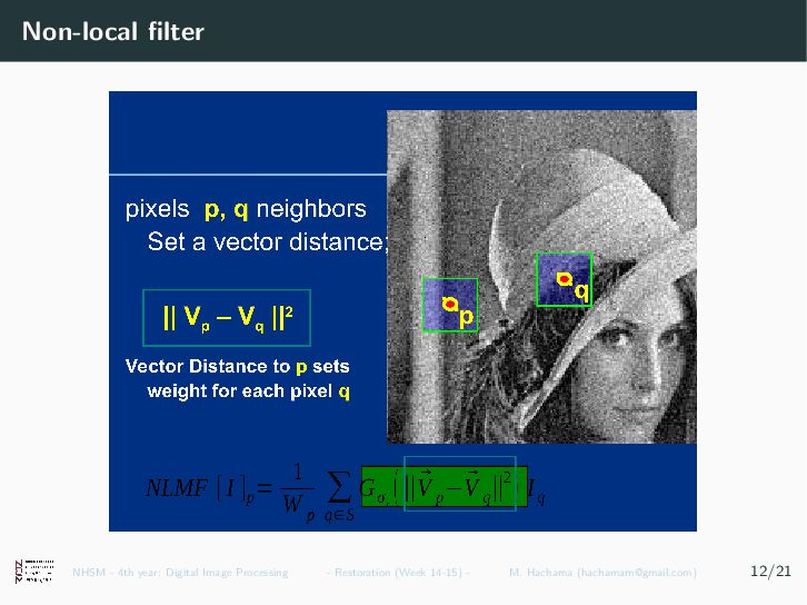
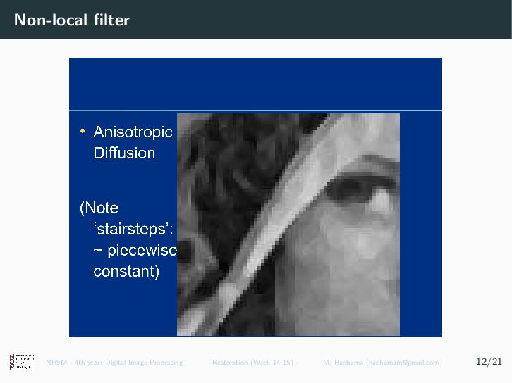
    • Bilateral: neighboring pixels with similar intensities • NL-Means: pixels with similar neighborhoods NHSM - 4th year: Digital Image Processing - Restoration (Week 14-15) - M. Hachama ([email protected]) 12/21
  40. Wiener filter • We know I0 (observed image) and σ

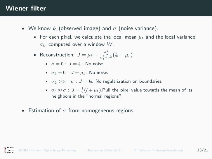
    (noise variance). • For each pixel, we calculate the local mean µL and the local variance σL , computed over a window W . • Reconstruction: J = µL + σ2 L σ2 L +σ2 (I0 − µL ) • σ = 0 : J = I0. No noise. • σL = 0 : J = µL . No noise. • σL >>= σ : J = I0. No regularization on boundaries. • σL ≈ σ : J = 1 2 (I + µL ).Pull the pixel value towards the mean of its neighbors in the ”normal regions”. • Estimation of σ from homogeneous regions. NHSM - 4th year: Digital Image Processing - Restoration (Week 14-15) - M. Hachama ([email protected]) 13/21
  41. Wiener filter • Example NHSM - 4th year: Digital Image

    Processing - Restoration (Week 14-15) - M. Hachama ([email protected]) 13/21
  42. Filtering • Frequency vs spatial filtering • Frequency filtering F(g)

    = HF(f ) NHSM - 4th year: Digital Image Processing - Restoration (Week 14-15) - M. Hachama ([email protected]) 15/21
  43. Low-pass filtering • Ideal low-pass filter NHSM - 4th year:

    Digital Image Processing - Restoration (Week 14-15) - M. Hachama ([email protected]) 16/21
  44. Low-pass filtering • Ideal low-pass filter NHSM - 4th year:

    Digital Image Processing - Restoration (Week 14-15) - M. Hachama ([email protected]) 16/21
  45. Low-pass filtering • Ideal low-pass filter NHSM - 4th year:

    Digital Image Processing - Restoration (Week 14-15) - M. Hachama ([email protected]) 16/21
  46. Low-pass filtering • Butterworth Low-pass filter NHSM - 4th year:

    Digital Image Processing - Restoration (Week 14-15) - M. Hachama ([email protected]) 16/21
  47. Filtering of a periodic noise • Input NHSM - 4th

    year: Digital Image Processing - Restoration (Week 14-15) - M. Hachama ([email protected]) 17/21
  48. Filtering of a periodic noise • Fourier transform NHSM -

    4th year: Digital Image Processing - Restoration (Week 14-15) - M. Hachama ([email protected]) 17/21
  49. Filtering of a periodic noise • Fourier transform NHSM -

    4th year: Digital Image Processing - Restoration (Week 14-15) - M. Hachama ([email protected]) 17/21
  50. Filtering of a periodic noise • Notch filter NHSM -

    4th year: Digital Image Processing - Restoration (Week 14-15) - M. Hachama ([email protected]) 17/21
  51. Filtering of a periodic noise • Frequency filtering NHSM -

    4th year: Digital Image Processing - Restoration (Week 14-15) - M. Hachama ([email protected]) 17/21
  52. Filtering of a periodic noise NHSM - 4th year: Digital

    Image Processing - Restoration (Week 14-15) - M. Hachama ([email protected]) 17/21
  53. Morphological filtering • Application to binary and grayscale images •

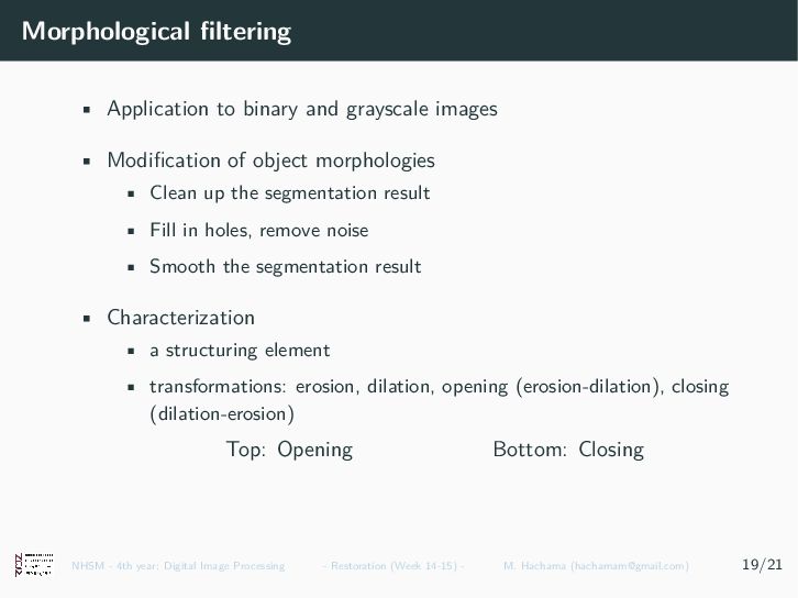
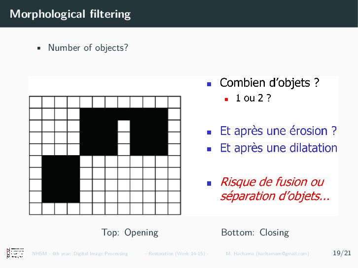
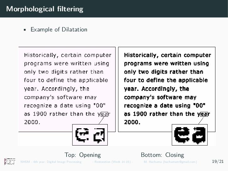
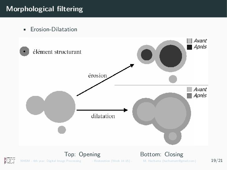
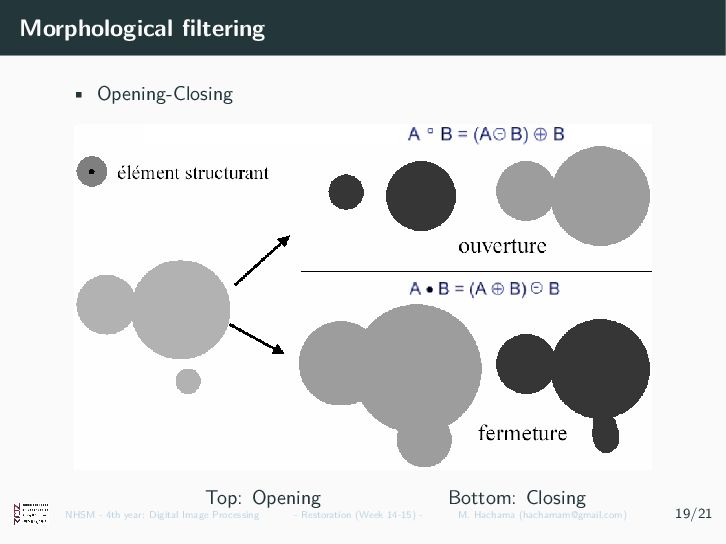
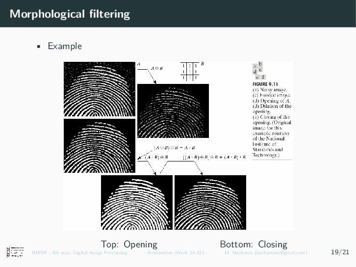
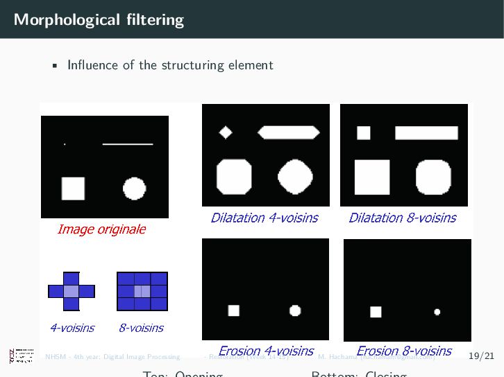
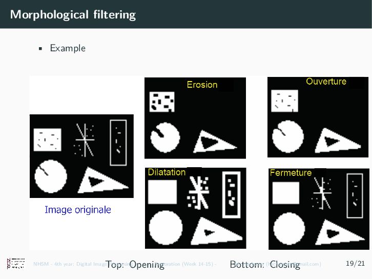
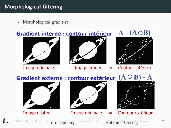
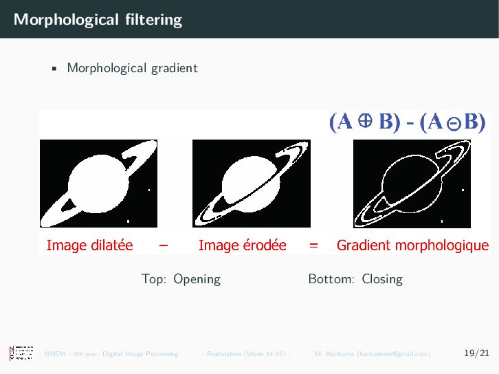
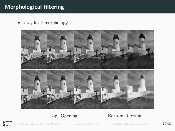
    Modification of object morphologies • Clean up the segmentation result • Fill in holes, remove noise • Smooth the segmentation result • Characterization • a structuring element • transformations: erosion, dilation, opening (erosion-dilation), closing (dilation-erosion) Top: Opening Bottom: Closing NHSM - 4th year: Digital Image Processing - Restoration (Week 14-15) - M. Hachama ([email protected]) 19/21
  54. Morphological filtering • Consider a binary image with background=0 and

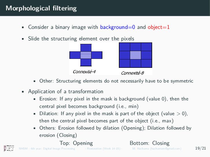
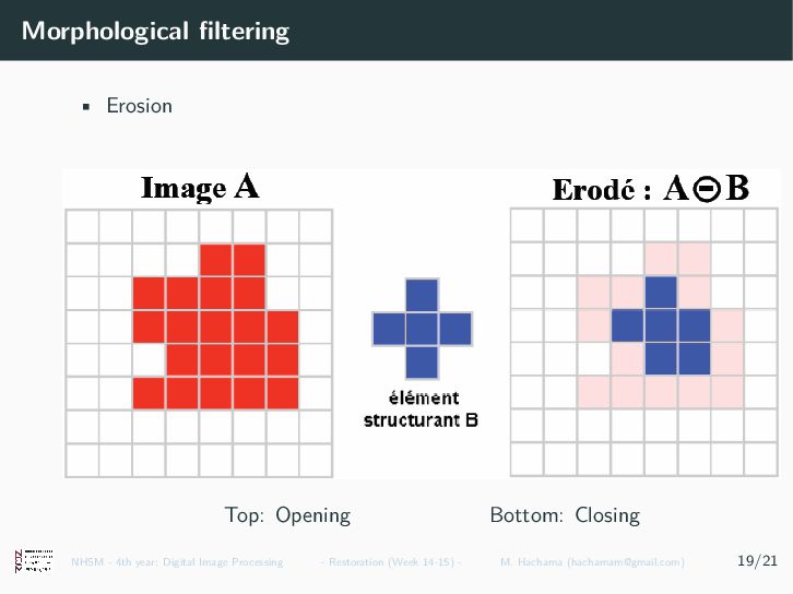
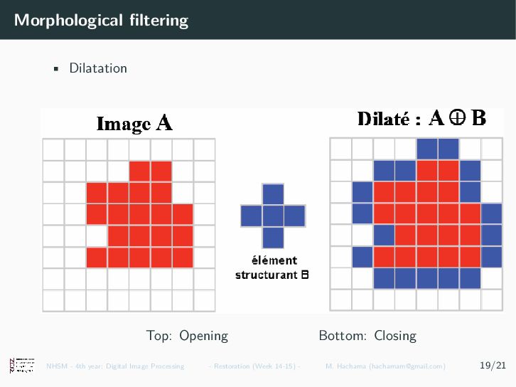
    object=1 • Slide the structuring element over the pixels • Other: Structuring elements do not necessarily have to be symmetric • Application of a transformation • Erosion: If any pixel in the mask is background (value 0), then the central pixel becomes background (i.e., min) • Dilation: If any pixel in the mask is part of the object (value > 0), then the central pixel becomes part of the object (i.e., max) • Others: Erosion followed by dilation (Opening); Dilation followed by erosion (Closing) Top: Opening Bottom: Closing NHSM - 4th year: Digital Image Processing - Restoration (Week 14-15) - M. Hachama ([email protected]) 19/21
  55. Morphological filtering • Erosion Top: Opening Bottom: Closing NHSM -

    4th year: Digital Image Processing - Restoration (Week 14-15) - M. Hachama ([email protected]) 19/21
  56. Morphological filtering • Dilatation Top: Opening Bottom: Closing NHSM -

    4th year: Digital Image Processing - Restoration (Week 14-15) - M. Hachama ([email protected]) 19/21
  57. Morphological filtering • Number of objects? Top: Opening Bottom: Closing

    NHSM - 4th year: Digital Image Processing - Restoration (Week 14-15) - M. Hachama ([email protected]) 19/21
  58. Morphological filtering • Example of Dilatation Top: Opening Bottom: Closing

    NHSM - 4th year: Digital Image Processing - Restoration (Week 14-15) - M. Hachama ([email protected]) 19/21
  59. Morphological filtering • Erosion-Dilatation Top: Opening Bottom: Closing NHSM -

    4th year: Digital Image Processing - Restoration (Week 14-15) - M. Hachama ([email protected]) 19/21
  60. Morphological filtering • Opening-Closing Top: Opening Bottom: Closing NHSM -

    4th year: Digital Image Processing - Restoration (Week 14-15) - M. Hachama ([email protected]) 19/21
  61. Morphological filtering • Example Top: Opening Bottom: Closing NHSM -

    4th year: Digital Image Processing - Restoration (Week 14-15) - M. Hachama ([email protected]) 19/21
  62. Morphological filtering • Influence of the structuring element NHSM -

    4th year: Digital Image Processing - Restoration (Week 14-15) - M. Hachama ([email protected]) 19/21
  63. Morphological filtering • Example Top: Opening Bottom: Closing NHSM -

    4th year: Digital Image Processing - Restoration (Week 14-15) - M. Hachama ([email protected]) 19/21
  64. Morphological filtering • Morphological gradient Top: Opening Bottom: Closing NHSM

    - 4th year: Digital Image Processing - Restoration (Week 14-15) - M. Hachama ([email protected]) 19/21
  65. Morphological filtering • Morphological gradient Top: Opening Bottom: Closing NHSM

    - 4th year: Digital Image Processing - Restoration (Week 14-15) - M. Hachama ([email protected]) 19/21
  66. Morphological filtering • Gray-level morphology Top: Opening Bottom: Closing NHSM

    - 4th year: Digital Image Processing - Restoration (Week 14-15) - M. Hachama ([email protected]) 19/21
  67. Inverse Filter • Degradation modeling: I0 = I ∗ h

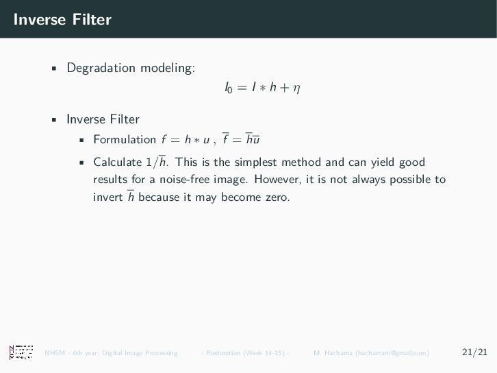
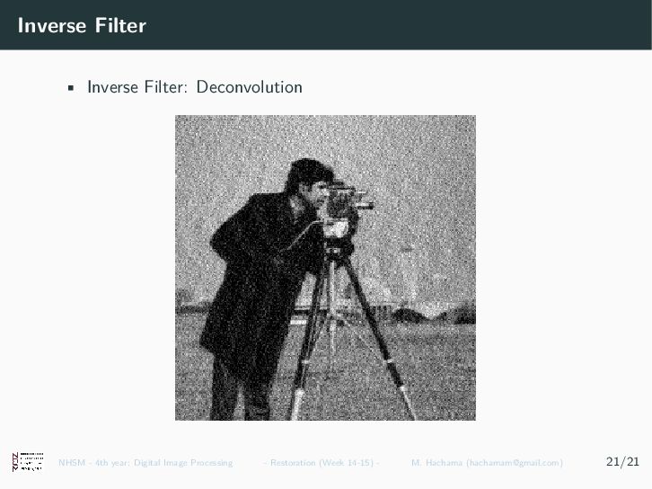
    + η • Inverse Filter • Formulation f = h ∗ u , f = hu • Calculate 1/h. This is the simplest method and can yield good results for a noise-free image. However, it is not always possible to invert h because it may become zero. NHSM - 4th year: Digital Image Processing - Restoration (Week 14-15) - M. Hachama ([email protected]) 21/21
  68. Inverse Filter • Inverse Filter: Deconvolution NHSM - 4th year:

    Digital Image Processing - Restoration (Week 14-15) - M. Hachama ([email protected]) 21/21
  69. Inverse Filter • Inverse Filter: Blurred image + Noise NHSM

    - 4th year: Digital Image Processing - Restoration (Week 14-15) - M. Hachama ([email protected]) 21/21
  70. Inverse Filter • Inverse Filter: Deconvolution NHSM - 4th year:

    Digital Image Processing - Restoration (Week 14-15) - M. Hachama ([email protected]) 21/21
  71. Inverse Filter Van Cittert Algorithm • Formulation f = h

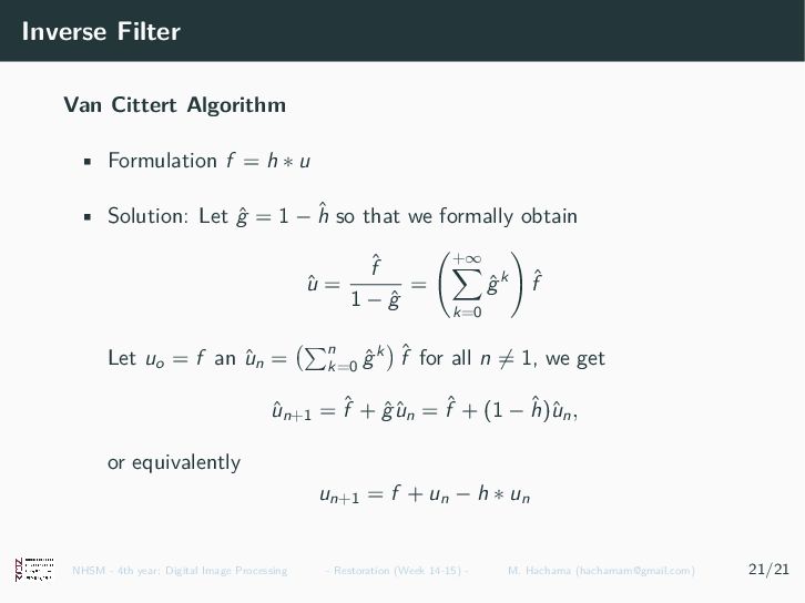
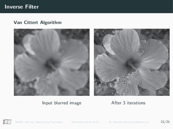
    ∗ u • Solution: Let ˆ g = 1 − ˆ h so that we formally obtain ˆ u = ˆ f 1 − ˆ g = +∞ k=0 ˆ gk ˆ f Let uo = f an ˆ un = n k=0 ˆ gk ˆ f for all n ̸= 1, we get ˆ un+1 = ˆ f + ˆ gˆ un = ˆ f + (1 − ˆ h)ˆ un, or equivalently un+1 = f + un − h ∗ un NHSM - 4th year: Digital Image Processing - Restoration (Week 14-15) - M. Hachama ([email protected]) 21/21
  72. Inverse Filter Van Cittert Algorithm Input blurred image After 3

    iterations NHSM - 4th year: Digital Image Processing - Restoration (Week 14-15) - M. Hachama ([email protected]) 21/21