to Pixel coordinates Camera calibration 3d vision 3D Reconstruction Stereo vision Binocular stereo NHSM - 4th year: Computer vision - 3d (Week 7-10) - M. Hachama ([email protected]) 3/19
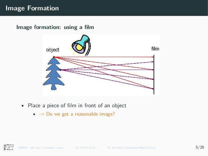
piece of film in front of an object • → Do we get a reasonable image? NHSM - 4th year: Computer vision - 3d (Week 7-10) - M. Hachama ([email protected]) 4/19
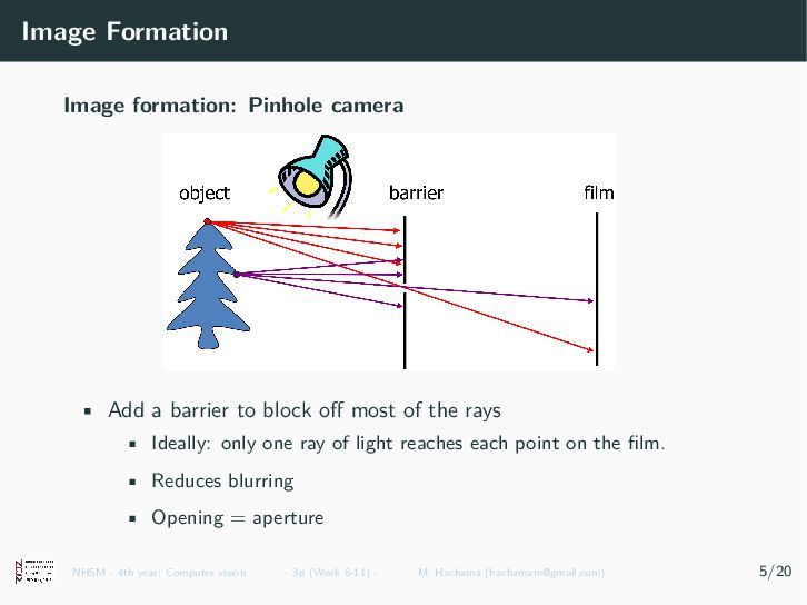
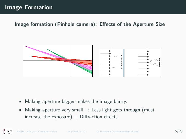
to block off most of the rays • Ideally: only one ray of light reaches each point on the film. • Reduces blurring • Opening = aperture NHSM - 4th year: Computer vision - 3d (Week 7-10) - M. Hachama ([email protected]) 4/19
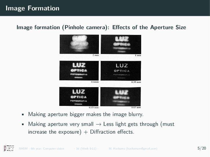
Size • Making aperture bigger makes the image blurry. • Making aperture very small → Less light gets through (must increase the exposure) + Diffraction effects. NHSM - 4th year: Computer vision - 3d (Week 7-10) - M. Hachama ([email protected]) 4/19
Size • Making aperture bigger makes the image blurry. • Making aperture very small → Less light gets through (must increase the exposure) + Diffraction effects. NHSM - 4th year: Computer vision - 3d (Week 7-10) - M. Hachama ([email protected]) 4/19
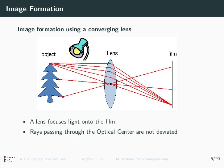
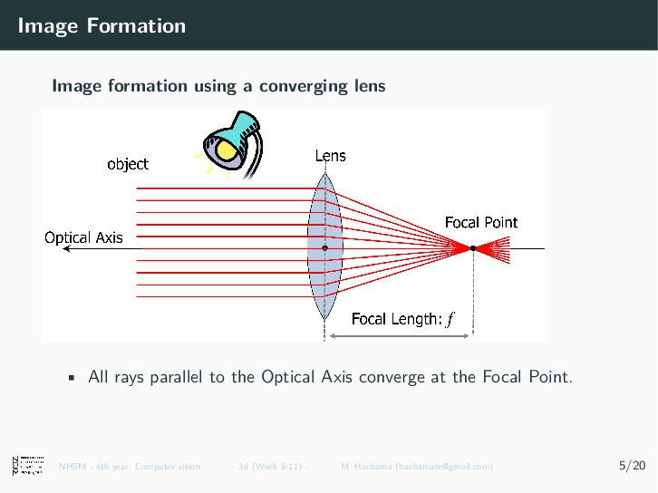
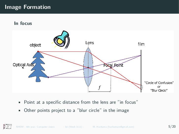
lens focuses light onto the film • Rays passing through the Optical Center are not deviated NHSM - 4th year: Computer vision - 3d (Week 7-10) - M. Hachama ([email protected]) 4/19
from the lens are ”in focus” • Other points project to a ”blur circle” in the image NHSM - 4th year: Computer vision - 3d (Week 7-10) - M. Hachama ([email protected]) 4/19
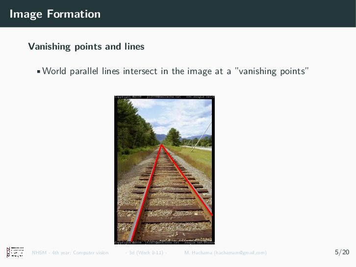
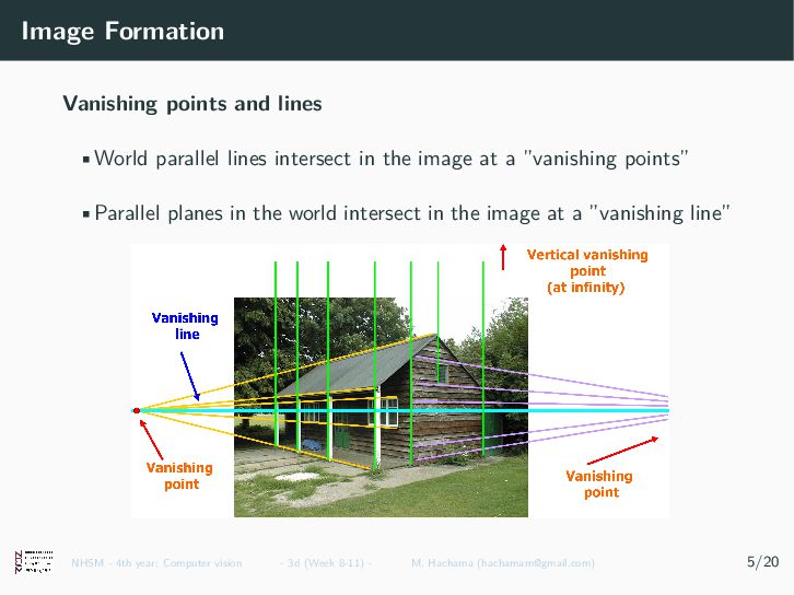
in the image at a ”vanishing points” •Parallel planes in the world intersect in the image at a ”vanishing line” NHSM - 4th year: Computer vision - 3d (Week 7-10) - M. Hachama ([email protected]) 4/19
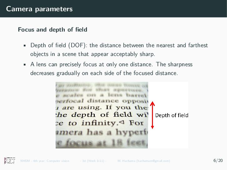
field (DOF): the distance between the nearest and farthest objects in a scene that appear acceptably sharp. • A lens can precisely focus at only one distance. The sharpness decreases gradually on each side of the focused distance. NHSM - 4th year: Computer vision - 3d (Week 7-10) - M. Hachama ([email protected]) 5/19
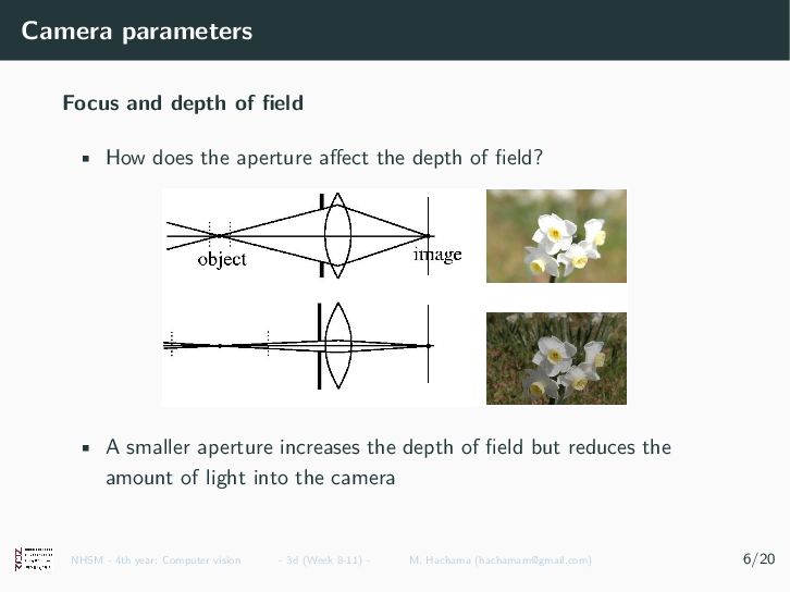
the aperture affect the depth of field? • A smaller aperture increases the depth of field but reduces the amount of light into the camera NHSM - 4th year: Computer vision - 3d (Week 7-10) - M. Hachama ([email protected]) 5/19
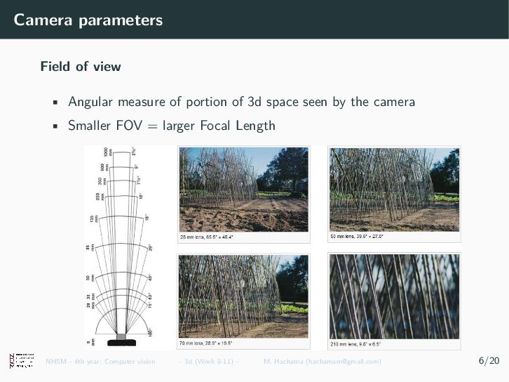
of 3d space seen by the camera • Smaller FOV = larger Focal Length NHSM - 4th year: Computer vision - 3d (Week 7-10) - M. Hachama ([email protected]) 5/19
to Pixel coordinates Camera calibration 3d vision 3D Reconstruction Stereo vision Binocular stereo NHSM - 4th year: Computer vision - 3d (Week 7-10) - M. Hachama ([email protected]) 6/19
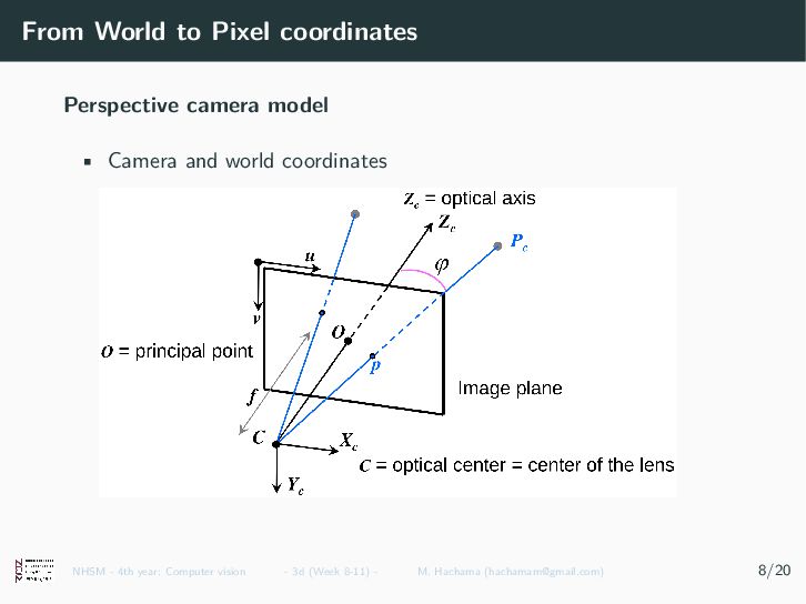
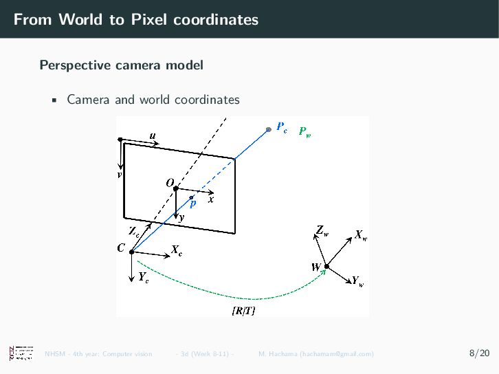
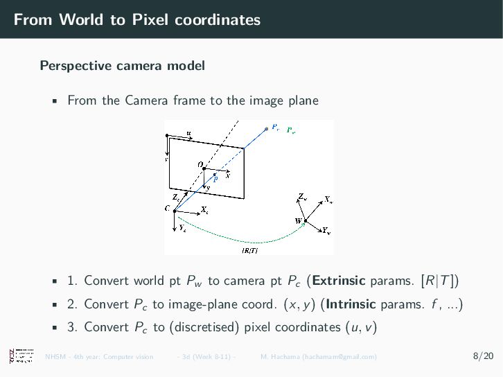
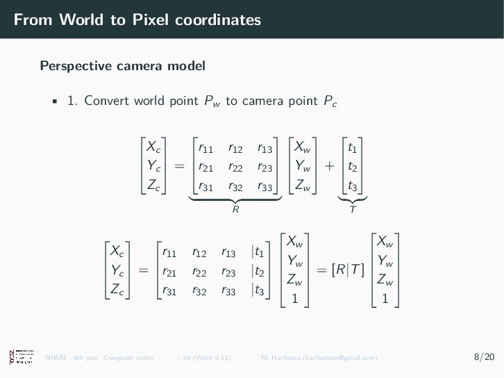
the Camera frame to the image plane • 1. Convert world pt Pw to camera pt Pc (Extrinsic params. [R|T]) • 2. Convert Pc to image-plane coord. (x, y) (Intrinsic params. f , ...) • 3. Convert Pc to (discretised) pixel coordinates (u, v) NHSM - 4th year: Computer vision - 3d (Week 7-10) - M. Hachama ([email protected]) 7/19
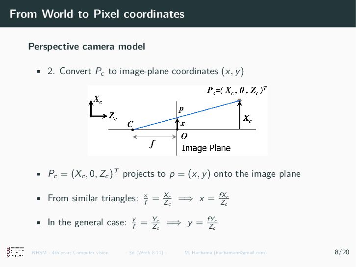
Convert Pc to image-plane coordinates (x, y) • Pc = (Xc , 0, Zc )T projects to p = (x, y) onto the image plane • From similar triangles: x f = Xc Zc =⇒ x = fXc Zc • In the general case: y f = Yc Zc =⇒ y = fYc Zc NHSM - 4th year: Computer vision - 3d (Week 7-10) - M. Hachama ([email protected]) 7/19
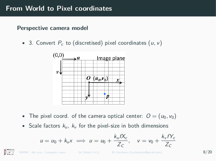
Convert Pc to (discretised) pixel coordinates (u, v) • The pixel coord. of the camera optical center: O = (u0, v0 ) • Scale factors ku , kv for the pixel-size in both dimensions u = u0 + ku x =⇒ u = u0 + ku fXc ZC , v = v0 + kv fYc ZC NHSM - 4th year: Computer vision - 3d (Week 7-10) - M. Hachama ([email protected]) 7/19
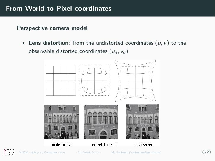
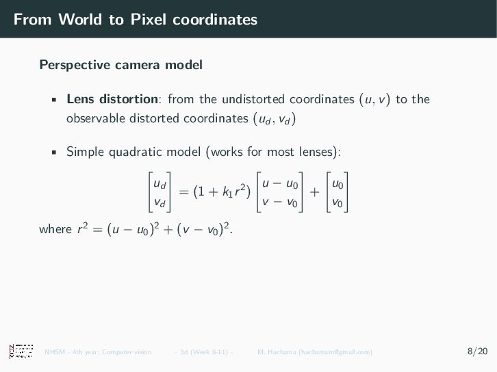
distortion: from the undistorted coordinates (u, v) to the observable distorted coordinates (ud , vd ) • Simple quadratic model (works for most lenses): ud vd = (1 + k1 r2) u − u0 v − v0 + u0 v0 where r2 = (u − u0 )2 + (v − v0 )2. NHSM - 4th year: Computer vision - 3d (Week 7-10) - M. Hachama ([email protected]) 7/19
to Pixel coordinates Camera calibration 3d vision 3D Reconstruction Stereo vision Binocular stereo NHSM - 4th year: Computer vision - 3d (Week 7-10) - M. Hachama ([email protected]) 8/19
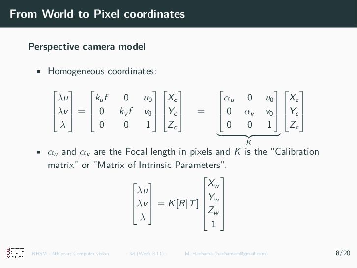
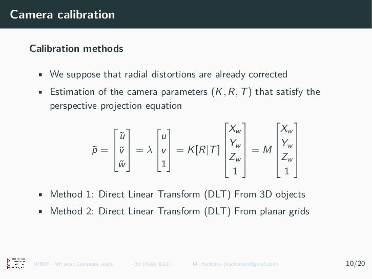
are already corrected • Estimation of the camera parameters (K, R, T) that satisfy the perspective projection equation ˜ p = ˜ u ˜ v ˜ w = λ u v 1 = K[R|T] Xw Yw Zw 1 = M Xw Yw Zw 1 • Method 1: Direct Linear Transform (DLT) From 3D objects • Method 2: Direct Linear Transform (DLT) From planar grids NHSM - 4th year: Computer vision - 3d (Week 7-10) - M. Hachama ([email protected]) 9/19
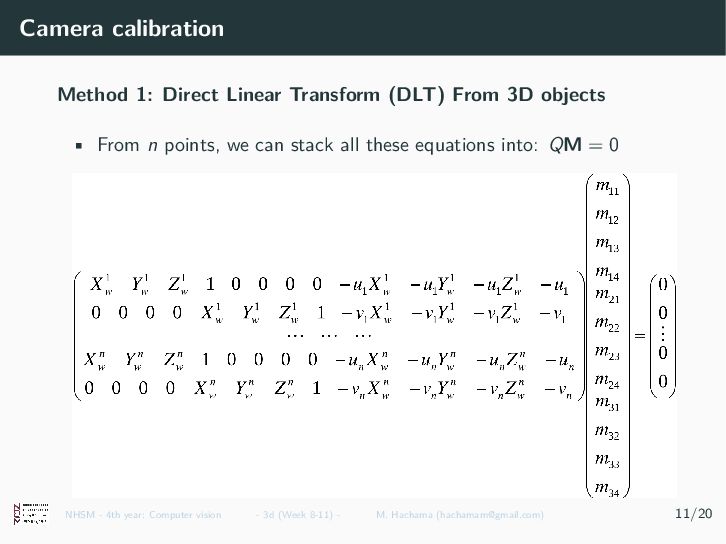
objects • From n points, we can stack all these equations into: QM = 0 NHSM - 4th year: Computer vision - 3d (Week 7-10) - M. Hachama ([email protected]) 10/19
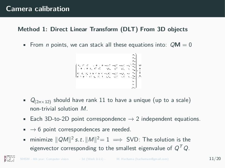
objects • From n points, we can stack all these equations into: QM = 0 • Q(2n×12) should have rank 11 to have a unique (up to a scale) non-trivial solution M. • Each 3D-to-2D point correspondence → 2 independent equations. • → 6 point correspondences are needed. • minimize ∥QM∥2 s.t. ∥M∥2= 1 =⇒ SVD: The solution is the eigenvector corresponding to the smallest eigenvalue of QT Q. NHSM - 4th year: Computer vision - 3d (Week 7-10) - M. Hachama ([email protected]) 10/19
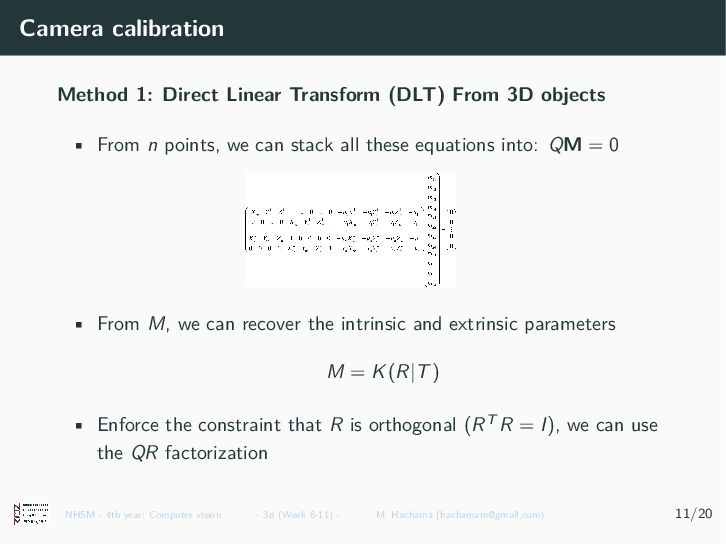
objects • From n points, we can stack all these equations into: QM = 0 • From M, we can recover the intrinsic and extrinsic parameters M = K(R|T) • Enforce the constraint that R is orthogonal (RT R = I), we can use the QR factorization NHSM - 4th year: Computer vision - 3d (Week 7-10) - M. Hachama ([email protected]) 10/19
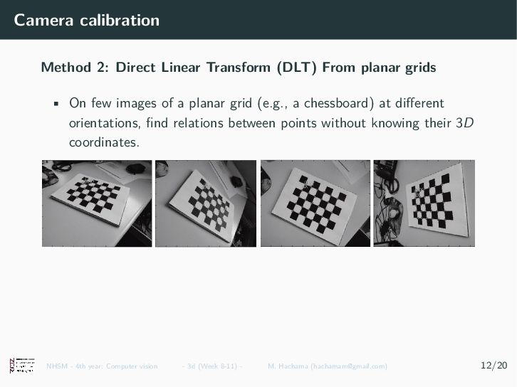
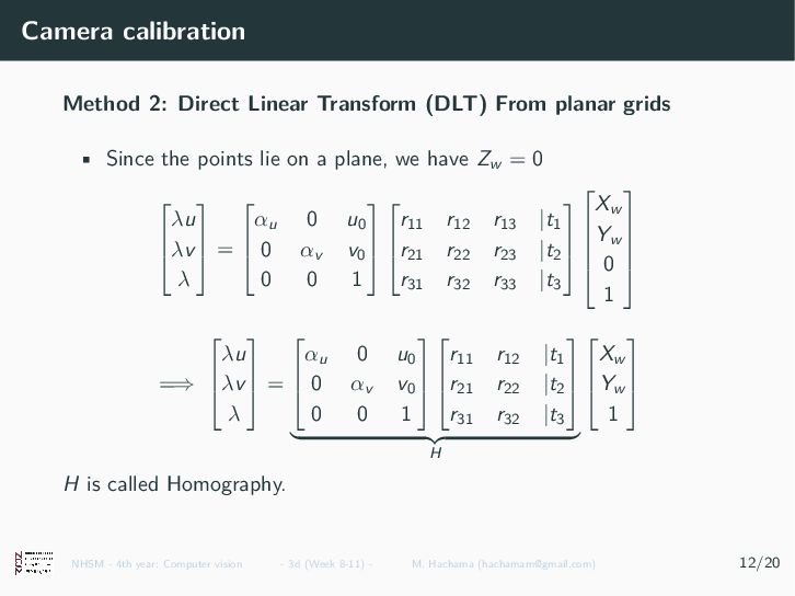
grids • On few images of a planar grid (e.g., a chessboard) at different orientations, find relations between points without knowing their 3D coordinates. NHSM - 4th year: Computer vision - 3d (Week 7-10) - M. Hachama ([email protected]) 11/19
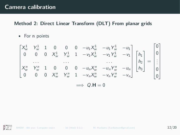
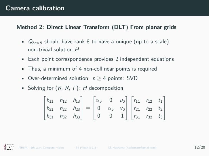
grids • For n points X1 w Y 1 w 1 0 0 0 −u1 X1 w −u1 Y 1 w −u1 0 0 0 X1 w Y 1 w 1 −v1 X1 w −v1 Y 1 w −v1 . . . . . . . . . Xn w Y n w 1 0 0 0 −un Xn w −un Y n w −un 0 0 0 Xn w Y n w 1 −vn Xn w −vn Y n w −vn h1 h2 h3 = 0 0 . . . 0 0 =⇒ Q.H = 0 NHSM - 4th year: Computer vision - 3d (Week 7-10) - M. Hachama ([email protected]) 11/19
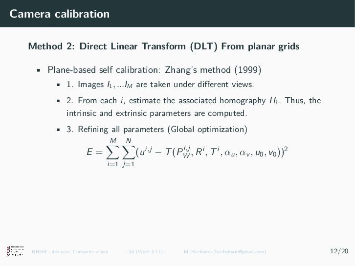
grids • Plane-based self calibration: Zhang’s method (1999) • 1. Images I1, ...IM are taken under different views. • 2. From each i, estimate the associated homography Hi . Thus, the intrinsic and extrinsic parameters are computed. • 3. Refining all parameters (Global optimization) E = M i=1 N j=1 (ui,j − T(Pi,j W , Ri , Ti , αu, αv , u0, v0 ))2 NHSM - 4th year: Computer vision - 3d (Week 7-10) - M. Hachama ([email protected]) 11/19
to Pixel coordinates Camera calibration 3d vision 3D Reconstruction Stereo vision Binocular stereo NHSM - 4th year: Computer vision - 3d (Week 7-10) - M. Hachama ([email protected]) 13/19
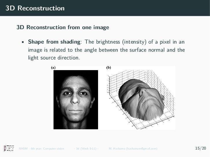
shading: The brightness (intensity) of a pixel in an image is related to the angle between the surface normal and the light source direction. NHSM - 4th year: Computer vision - 3d (Week 7-10) - M. Hachama ([email protected]) 14/19
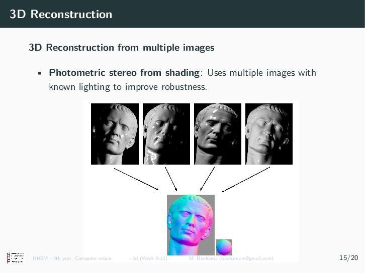
from shading: Uses multiple images with known lighting to improve robustness. NHSM - 4th year: Computer vision - 3d (Week 7-10) - M. Hachama ([email protected]) 14/19
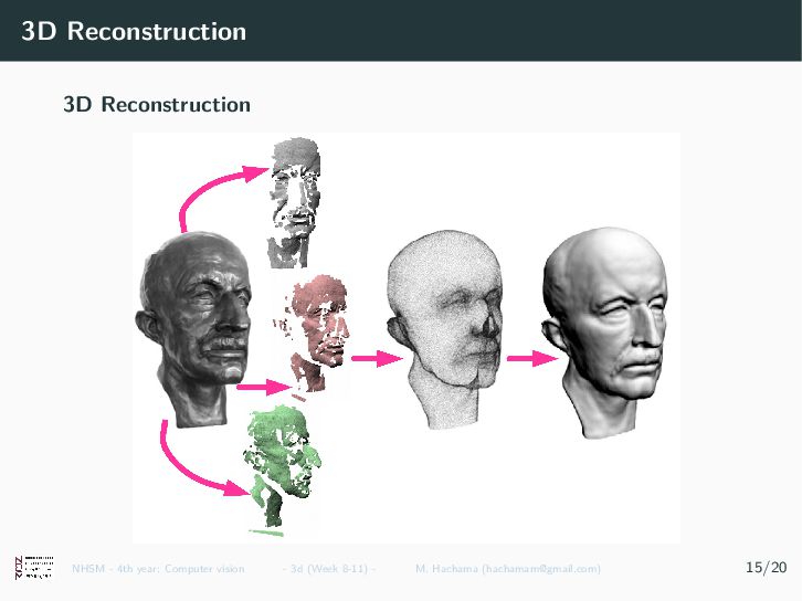
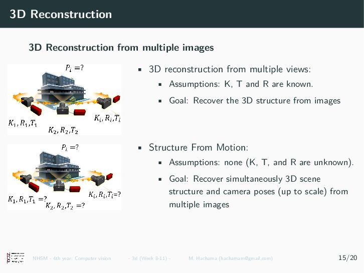
from multiple views: • Assumptions: K, T and R are known. • Goal: Recover the 3D structure from images • Structure From Motion: • Assumptions: none (K, T, and R are unknown). • Goal: Recover simultaneously 3D scene structure and camera poses (up to scale) from multiple images NHSM - 4th year: Computer vision - 3d (Week 7-10) - M. Hachama ([email protected]) 14/19
to Pixel coordinates Camera calibration 3d vision 3D Reconstruction Stereo vision Binocular stereo NHSM - 4th year: Computer vision - 3d (Week 7-10) - M. Hachama ([email protected]) 15/19
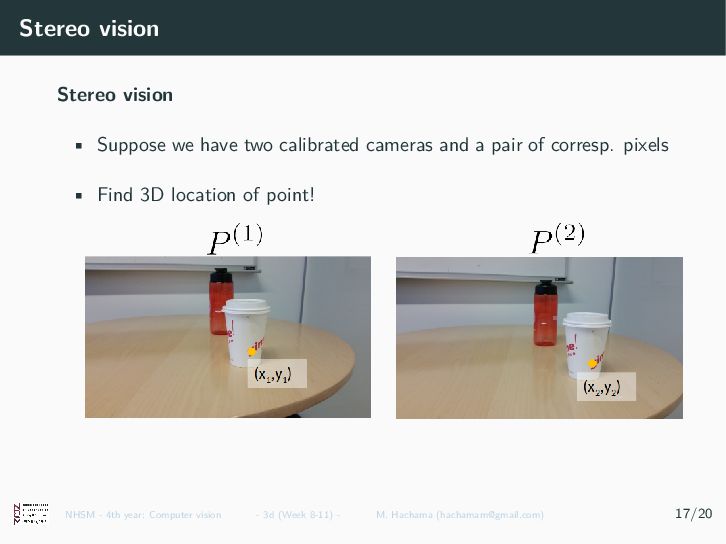
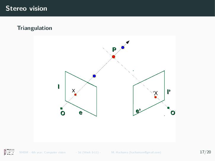
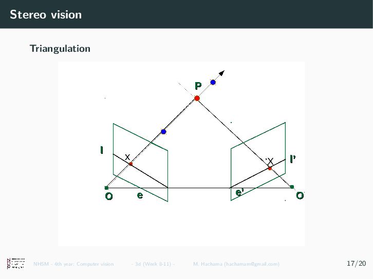
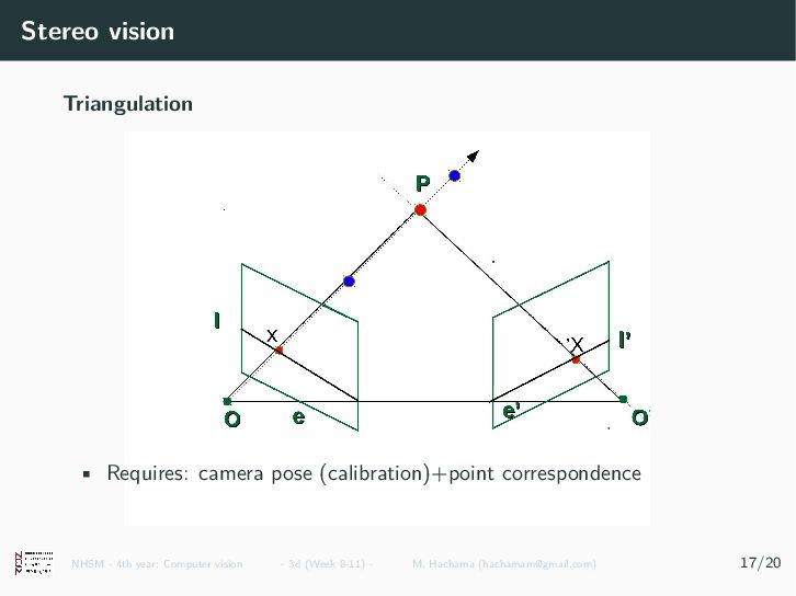
cameras and a pair of corresp. pixels • Find 3D location of point! NHSM - 4th year: Computer vision - 3d (Week 7-10) - M. Hachama ([email protected]) 16/19
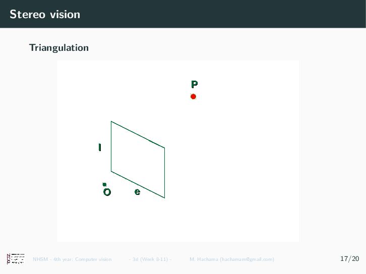
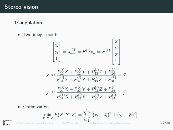
xi yi 1 = x(1) img = P(1)xw = P(1) X Y Z 1 xi ≈ P(i) 11 X + P(i) 12 Y + P(i) 13 Z + P(i) 14 P(i) 31 X + P(i) 32 Y + P(i) 33 Z + P(1) 34 = ¯ xi yi ≈ P(i) 21 X + P(i) 22 Y + P(i) 23 Z + P(i) 24 P(1) 31 X + P(i) 32 Y + P(i) 33 Z + P(i) 34 = ¯ yi • Optimization min X,Y ,Z E(X, Y , Z) = 2 i=1 (xi − ¯ xi )2 + (yi − ¯ yi )2 . NHSM - 4th year: Computer vision - 3d (Week 7-10) - M. Hachama ([email protected]) 16/19
to Pixel coordinates Camera calibration 3d vision 3D Reconstruction Stereo vision Binocular stereo NHSM - 4th year: Computer vision - 3d (Week 7-10) - M. Hachama ([email protected]) 17/19
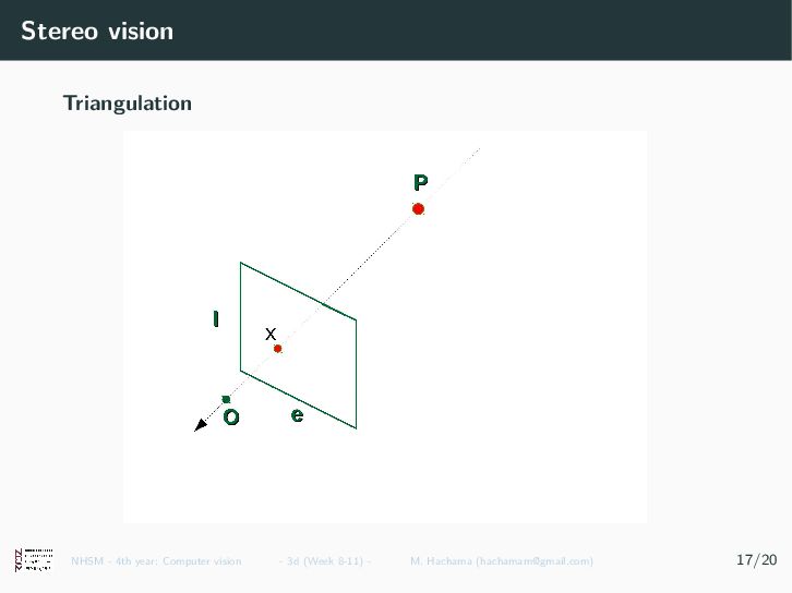
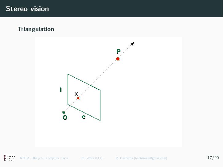
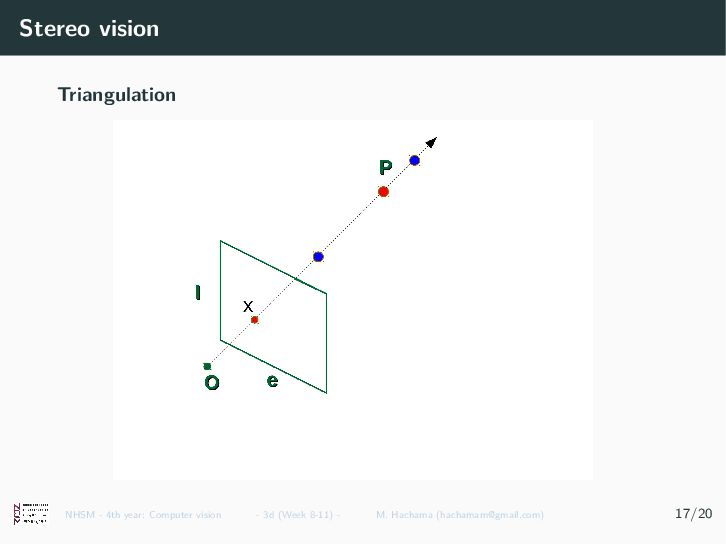
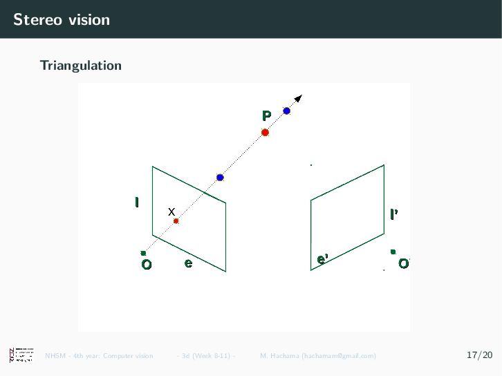
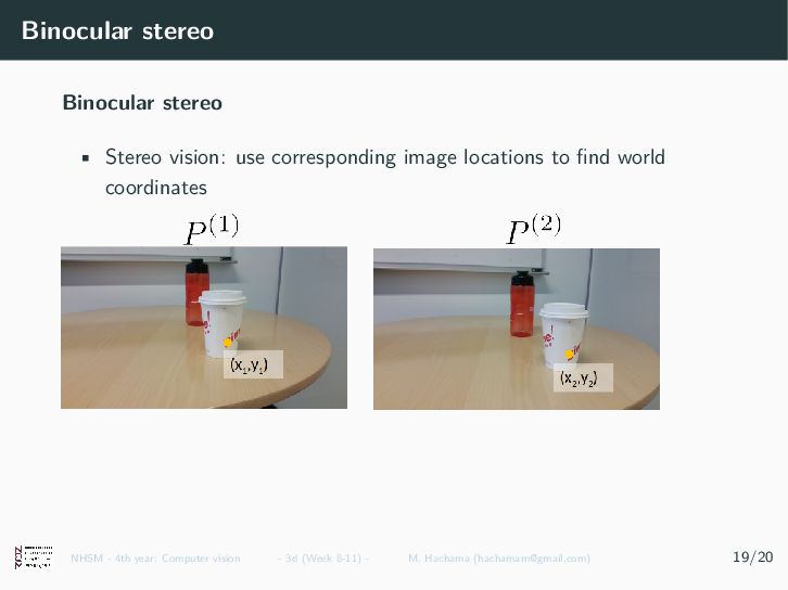
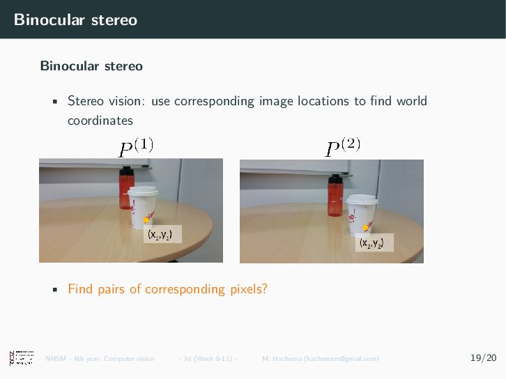
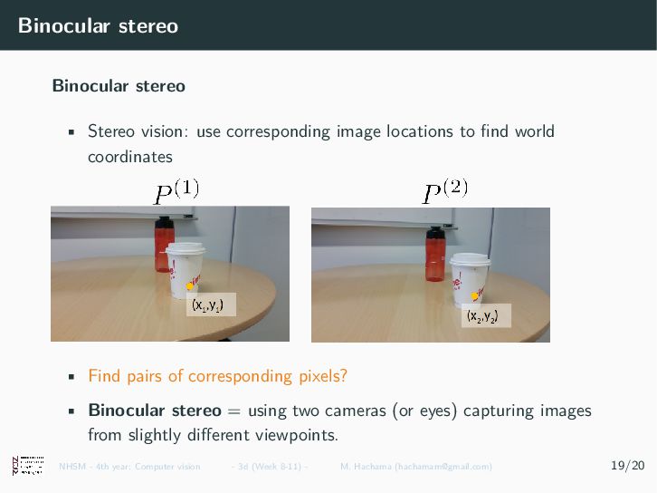
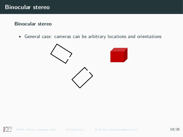
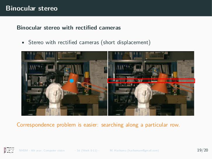
locations to find world coordinates • Find pairs of corresponding pixels? • Binocular stereo = using two cameras (or eyes) capturing images from slightly different viewpoints. NHSM - 4th year: Computer vision - 3d (Week 7-10) - M. Hachama ([email protected]) 18/19
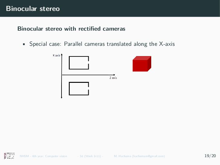
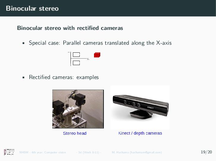
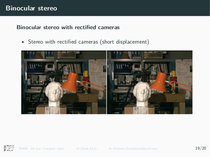
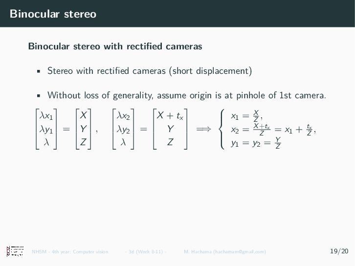
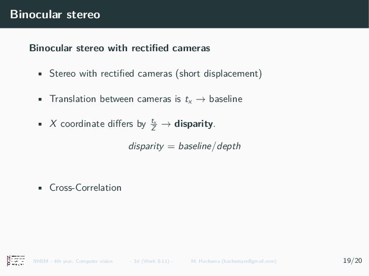
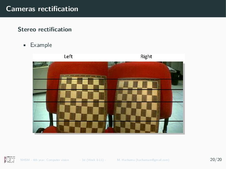
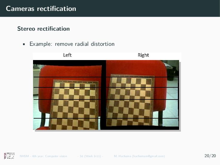
rectified cameras (short displacement) Correspondence problem is easier: searching along a particular row. NHSM - 4th year: Computer vision - 3d (Week 7-10) - M. Hachama ([email protected]) 18/19
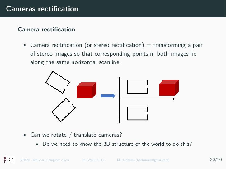
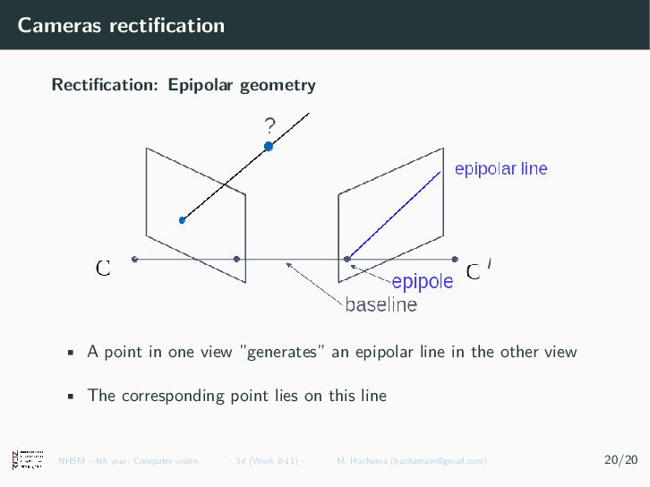
= transforming a pair of stereo images so that corresponding points in both images lie along the same horizontal scanline. • Can we rotate / translate cameras? • Do we need to know the 3D structure of the world to do this? NHSM - 4th year: Computer vision - 3d (Week 7-10) - M. Hachama ([email protected]) 19/19
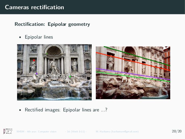
view ”generates” an epipolar line in the other view • The corresponding point lies on this line NHSM - 4th year: Computer vision - 3d (Week 7-10) - M. Hachama ([email protected]) 19/19