CV_1_Introduction

Computer vision Introduction (Week 1) NHSM - 4th year -
Spring 2026 - Prof. Mohammed Hachama [email protected] hachama.github.io/home

Introduction NHSM - 4th year: Computer vision - Introduction (Week
1) - M. Hachama ([email protected]) 2/21

Outline Introduction Computer vision Organization of the course Fitting and
alignment Matrix decomposition Least squares RANSAC Template matching NHSM - 4th year: Computer vision - Introduction (Week 1) - M. Hachama ([email protected]) 3/21

Extract ”information” from pixels Figure 1: What we see Figure
2: What computer sees NHSM - 4th year: Computer vision - Introduction (Week 1) - M. Hachama ([email protected]) 4/21

Extract ”information” from pixels Figure 1: Input Image NHSM -
4th year: Computer vision - Introduction (Week 1) - M. Hachama ([email protected]) 4/21

Extract ”information” from pixels Figure 1: Input Image Figure 2:
Geometric information NHSM - 4th year: Computer vision - Introduction (Week 1) - M. Hachama ([email protected]) 4/21

Extract ”information” from pixels Figure 1: Input Image Figure 2:
Semantic information NHSM - 4th year: Computer vision - Introduction (Week 1) - M. Hachama ([email protected]) 4/21

Industrial vision Optical character recognition (OCR) NHSM - 4th year:
Computer vision - Introduction (Week 1) - M. Hachama ([email protected]) 5/21

Industrial vision Visual inspection for quality assurance NHSM - 4th
year: Computer vision - Introduction (Week 1) - M. Hachama ([email protected]) 5/21

Computer animation Use of retro-reflective markers to capture actors motion
NHSM - 4th year: Computer vision - Introduction (Week 1) - M. Hachama ([email protected]) 5/21

Image edition Editing images as if they were 3D scenes
NHSM - 4th year: Computer vision - Introduction (Week 1) - M. Hachama ([email protected]) 5/21

Vision-based biometrics How the Afghan girl was Identified by Her
Iris Patterns NHSM - 4th year: Computer vision - Introduction (Week 1) - M. Hachama ([email protected]) 5/21

Information about the course • Image processing courses • Introduction
to image processing (S7 - UEF721): Image = matrix • Computer vision (S8 - UEF823): More applications • Image processing (S9 - UEF911): Image = function (more elaborated mathematics: PDEs+Variational Calculus) NHSM - 4th year: Computer vision - Introduction (Week 1) - M. Hachama ([email protected]) 7/21

to image processing (S7 - UEF721): Image = matrix • Computer vision (S8 - UEF823): More applications • Image processing (S9 - UEF911): Image = function (more elaborated mathematics: PDEs+Variational Calculus) • UEF823 Course • 1 Lecture: slides, no written notes (see references if need be!) • 1 Tutorial/Practical session • 6 Chapters: 1 assignment + 1 Lab session + 1 Quiz • 1 Project NHSM - 4th year: Computer vision - Introduction (Week 1) - M. Hachama ([email protected]) 7/21

to image processing (S7 - UEF721): Image = matrix • Computer vision (S8 - UEF823): More applications • Image processing (S9 - UEF911): Image = function (more elaborated mathematics: PDEs+Variational Calculus) • UEF823 Course • 1 Lecture: slides, no written notes (see references if need be!) • 1 Tutorial/Practical session • 6 Chapters: 1 assignment + 1 Lab session + 1 Quiz • 1 Project • Evaluation • Grade = Final Exam (20) + Midterm (10) + Project (10) + Bonus • Bonus = HWs (3) → Submission one week after midterm • After two absences: -1 point for each additional absence NHSM - 4th year: Computer vision - Introduction (Week 1) - M. Hachama ([email protected]) 7/21

Information about the course • Syllabus: 15 weeks • Introduction
(1 week) • Pyramidal representations (1 week) • Key-points description and extraction (3 weeks) • Motion estimation (1 week) • Mid-Term • 3D vision (4 weeks) • Deep learning (4 weeks) • Evaluations (projects) (1 week) • Links • Course: hachama.github.io/vision • Canvas: canvas.instructure.com/courses/11329701 • Professor: hachama.github.io/home NHSM - 4th year: Computer vision - Introduction (Week 1) - M. Hachama ([email protected]) 7/21

Information about the course • Books • Computer Vision: Algorithms
and Applications. • Computer vision, A modern approach. • Concise Computer Vision, An Introd. into Theo. and Alg. • Advanced Image and Video Processing Using MATLAB. • Hands-On Image Processing with Python. NHSM - 4th year: Computer vision - Introduction (Week 1) - M. Hachama ([email protected]) 7/21

Information about the course • Similar courses • CS 131
Computer Vision: Foundations and Applications (Stanford University) • Introduction to Computer Vision, CS5670, Spring 2023, Cornell Tech, www.cs.cornell.edu/courses/cs5670/2024sp/ • 16-385 Computer Vision, Spring 2020, Carnegie Mellon, www.cs.cmu.edu/∼16385/ • YouTube lectures • Image and video Processing: From Mars to Hollywood with a Strop at the Hospital, Guillermo Sapiro • Intro to Digital Image Processing, Rich Radke • Various codes • www.numerical-tours.com NHSM - 4th year: Computer vision - Introduction (Week 1) - M. Hachama ([email protected]) 7/21

Fitting and alignment NHSM - 4th year: Computer vision -
Introduction (Week 1) - M. Hachama ([email protected]) 8/21

Factorization SVD • Any matrix X can be decomposed as
Xn×p = Un×n Σn×p V T p×p , • U, V are orthogonal and σ1 ≥ ... ≥ σr are the singular values. • Σ =      σ1 ... σr ⃝      or Σ =    σ1 ... ⃝ σr    . • Columns of V are normalized eigenvectors of XT X. • Columns of U are normalized eigenvectors of XXT . • uj and vj share the same eigenvalue λj , where σj = λj . • Every matrix X of rank r has exactly r nonzero singular values. NHSM - 4th year: Computer vision - Introduction (Week 1) - M. Hachama ([email protected]) 10/21

Factorization SVD • Full and compact (reduced) SVD • Full
SVD: X = UΣV T • Compact SVD: X = U1 Σ1V T 1 , i.e., X = r i=1 σi ui vT i . NHSM - 4th year: Computer vision - Introduction (Week 1) - M. Hachama ([email protected]) 10/21

Computing the compact SVD Algorithm 1 1: procedure compact SVD(A)
2: λ, V ← eig(AT A) ▷ Calculate the eigenvalues and eigenvectors of AT A. 3: σ ← √ λ ▷ Calculate the singular values of A. 4: σ ← sort(σ) ▷ Sort the singular values from greatest to least. 5: V ← sort(V ) ▷ Sort the eigenvectors the same way. 6: r ← count(σ ̸= 0) ▷ Count the number of nonzero singular values (the rank of A). 7: σ1 ← σ:r ▷ Keep only the positive singular values. 8: V1 ← V:,:r ▷ Keep only the corresponding eigenvectors. 9: U1 ← AV1/σ1 ▷ Construct U with array broadcasting. 10: return U1, σ1, V T 1 11: end procedure NHSM - 4th year: Computer vision - Introduction (Week 1) - M. Hachama ([email protected]) 10/21

Factorization SVD • Intuition: X can be seen as a
linear transformation. This transformation can be decomposed in three sub-transformations: 1. Rotation, 2. Re-scaling, 3. Rotation. These three steps correspond to the three matrices U, D, and V. NHSM - 4th year: Computer vision - Introduction (Week 1) - M. Hachama ([email protected]) 10/21

Applications of SVD • The pseudoinverse of a rectangular matrix
X is X+ = V    σ−1 1 ... ⃝ σ−1 p    UT • X has linearly independent columns (XT X is invertible): X+ = (XT X)−1XT . In this case, X+X = I. • X has linearly independent rows (matrix XXT is invertible): X+ = XT (XXT )−1. This is a right inverse, as XX+ = I. NHSM - 4th year: Computer vision - Introduction (Week 1) - M. Hachama ([email protected]) 10/21

Applications of SVD • If A is a m ×
n matrix of rank r < min{m, n}, store the matrices U1 , Σ1 and V1 instead of A. • Store A: mn values • Store the matrices U1 , Σ1 and V1 : mr + r + nr values. • Example: If A is 100 × 200 and has rank 20 • Store A: 20, 000 values • Store the matrices U1 , Σ1 and V1 : 6, 020 entries. NHSM - 4th year: Computer vision - Introduction (Week 1) - M. Hachama ([email protected]) 10/21

Applications of SVD • The truncated SVD keeps only the
first s < r singular values, plus the corresponding columns of U and V : As = s i=1 σi ui vT i . The resulting matrix As has rank s and is only an approximation to A, since r − s nonzero singular values are neglected. NHSM - 4th year: Computer vision - Introduction (Week 1) - M. Hachama ([email protected]) 10/21

Applications of SVD NHSM - 4th year: Computer vision -

QR Factorization • Any matrix An×p with linearly independent columns
admits a unique decomposition An×p = Qn×p Rp×p where QT Q = I and R is upper triangular. • QR is a useful factorization when n > p. • Full QR decomposition A m×n = Q m×m R 0 m×n = Q1 Q2 R 0 m×n • Reduced QR decomposition A m×n = Q1 m×n R n×n NHSM - 4th year: Computer vision - Introduction (Week 1) - M. Hachama ([email protected]) 10/21

Least squares NHSM - 4th year: Computer vision - Introduction
(Week 1) - M. Hachama ([email protected]) 12/21

Total Least squares • Fitting a line to a point
cloud • Data: (x1, y1 ), ·, (xn, yn ) • Line equation: y = ax + b • Find (a, b) to minimize E(a, b) = n i=1 (yi − axi − b)2 NHSM - 4th year: Computer vision - Introduction (Week 1) - M. Hachama ([email protected]) 13/21

Total Least squares • Fitting a line to a point
cloud E(a, b) = n i=1 (yi − axi − b)2 = ||Ac − d||2 A =    x1 1 . . . . . . xn 1    ; c = a b ; d =    y1 . . . yn    • Cons • Fails for vertical lines • Not rotation-invariant NHSM - 4th year: Computer vision - Introduction (Week 1) - M. Hachama ([email protected]) 13/21

Total Least squares • Minimize the function min c∈Rn E(c)
, / E(c) = ∥Ac − d∥2 • The problem always has solution (size(A) = m × n). • Sol. is unique ⇔ rank(A) = n. • Resolution • Normal equations • Orthogonal methods • SVD NHSM - 4th year: Computer vision - Introduction (Week 1) - M. Hachama ([email protected]) 13/21

Total Least squares • Minimize the function min c∈Rn E(c)
, / E(c) = ∥Ac − d∥2 • EL: ∂E ∂c = 2(AT A)c − 2AT d = 0. • Normal equation AT A c = AT d. AT A c = AT d =⇒ c = A+d. when A has linearly independent columns and where A+ = (AT A)−1AT NHSM - 4th year: Computer vision - Introduction (Week 1) - M. Hachama ([email protected]) 13/21

Total Least squares • Solution using QR factorization A =
QR ˆ c = (AT A)−1AT d = ((QR)T (QR))−1(QR)T d = (RT QT QR)−1RT QT d = (RT R)−1RT QT d = R−1R−T RT Q−1d = R−1QT d • Algorithm • 1. compute QR factorization A = QR. • 2. matrix-vector product x = QT d • 3. solve Rc = x by back substitution NHSM - 4th year: Computer vision - Introduction (Week 1) - M. Hachama ([email protected]) 13/21

RANSAC NHSM - 4th year: Computer vision - Introduction (Week
1) - M. Hachama ([email protected]) 15/21

Robust estimation • Outliers are points that don’t ”fit” the
model. NHSM - 4th year: Computer vision - Introduction (Week 1) - M. Hachama ([email protected]) 16/21

Algorithm • RANSAC or “RANdom SAmple Consensus” an iterative method
to ”robustly” estimate parameters of a mathematical model from a set of observed data which contains outliers. • Untill N iterations have occured: • Draw a random sample of S points from the data • Fit the model to that set of S points • Classify data points as outliers or inliers • ReFit the model to inliers while ignoring outliers • Use the best fit from this collection using the fitting error. NHSM - 4th year: Computer vision - Introduction (Week 1) - M. Hachama ([email protected]) 16/21

Example: Line fitting NHSM - 4th year: Computer vision -

Example: Compute a mapping between two images • Several hundred
key-points extracted from each image need to be matched: compute the transf. which minimises a given criterion. • Outliers (incorrect matches) which will corrupt the estimation. • RANSAC: Choose a subset of the points from one image, match these to the other image and compute the transformation which minimises the re-projection error. Repeat using different subsets of key points each time. Then select the best transformation. NHSM - 4th year: Computer vision - Introduction (Week 1) - M. Hachama ([email protected]) 18/21

Template matching NHSM - 4th year: Computer vision - Introduction
(Week 1) - M. Hachama ([email protected]) 20/21

Template matching • Source image (I): The image in which
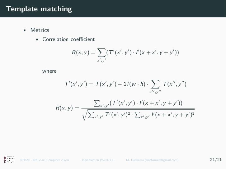
we expect to find a match to the template image • Template image (T): The patch image which will be compared to the template to detect the highest matching area NHSM - 4th year: Computer vision - Introduction (Week 1) - M. Hachama ([email protected]) 21/21

Template matching • Comparing the template against the source image
by sliding it • Moving the patch one pixel at a time. • At each location, a similarity metric is calculated NHSM - 4th year: Computer vision - Introduction (Week 1) - M. Hachama ([email protected]) 21/21

Template matching • Store the metric in the result matrix
(image) (R). NHSM - 4th year: Computer vision - Introduction (Week 1) - M. Hachama ([email protected]) 21/21

Template matching • Metrics • Sum of Square differences R(x,
y) = x′,y′ (T(x′, y′) − I(x + x′, y + y′))2 R(x, y) = x′,y′ (T(x′, y′) − I(x + x′, y + y′))2 x′,y′ T(x′, y′)2 · x′,y′ I(x + x′, y + y′)2 • Cross-correlation R(x, y) = x′,y′ (T(x′, y′) · I(x + x′, y + y′)) R(x, y) = x′,y′ (T(x′, y′) · I(x + x′, y + y′)) x′,y′ T(x′, y′)2 · x′,y′ I(x + x′, y + y′)2 NHSM - 4th year: Computer vision - Introduction (Week 1) - M. Hachama ([email protected]) 21/21

Template matching • Metrics • Correlation coefficient R(x, y) =
x′,y′ (T′(x′, y′) · I′(x + x′, y + y′)) where T′(x′, y′) = T(x′, y′) − 1/(w · h) · x′′,y′′ T(x′′, y′′) R(x, y) = x′,y′ (T′(x′, y′) · I′(x + x′, y + y′)) x′,y′ T′(x′, y′)2 · x′,y′ I′(x + x′, y + y′)2 NHSM - 4th year: Computer vision - Introduction (Week 1) - M. Hachama ([email protected]) 21/21

CV_1_Introduction

CV_1_Introduction

More Decks by Mohammed Hachama

Other Decks in Education

Featured

Transcript