EUSIPCO 2021

Stochastic permutation ordering watershed

Transcript

1. STOCHASTIC PERMUTATION ORDERING WATERSHED Olivier L´ EZORAY Normandie Univ, UNICAEN, ENSICAEN, CNRS, GREYC, Caen, FRANCE olivier.lezoray@unicaen.fr https://lezoray.users.greyc.fr
2. Graph Signals The domain Ω of the image is considered as a grid graph G = (V, E) Vertices V = {v1, . . . , vm} correspond to pixels Edges eij = (vi, vj) connect vertices with 8-adjacency Images are represented as graph signals where real-valued vectors are associated to vertices: f : G → T ⊂ Rn We consider the union of spectral and spatial graphs: -adjacency graphs and -nn graphs G20 ∪ G21 ∗ The set T = {v1, · · · , vm} represents all the vectors associated to all vertices To each vertex vi ∈ G is associated a vector f(vi) = vi = T [i] O. L´ ezoray Stochastic permutation ordering watershed /
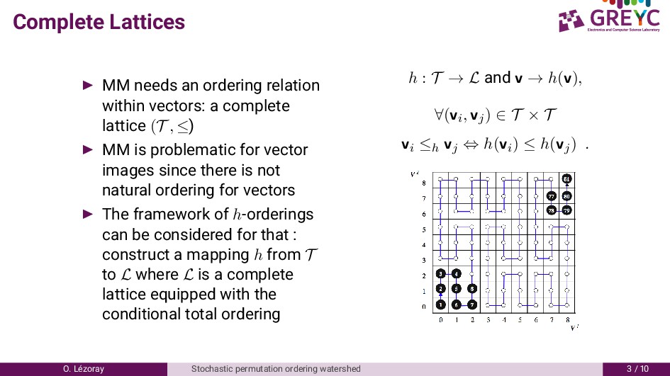
3. Complete Lattices MM needs an ordering relation within vectors: a complete lattice (T , ≤) MM is problematic for vector images since there is not natural ordering for vectors The framework of h-orderings can be considered for that : construct a mapping h from T to L where L is a complete lattice equipped with the conditional total ordering h : T → L and v → h(v), ∀(vi, vj) ∈ T × T vi ≤h vj ⇔ h(vi) ≤ h(vj) . O. L´ ezoray Stochastic permutation ordering watershed /
4. Stochastic Hamiltonian path Our proposal : construct a complete lattice with an image-adaptive h-ordering based on an Hamiltonian path Equivalent as defining a sorted permutation of the vectors of T is defined as P = PT with P a permutation matrix of size m × m Any permutation is not of interest, we search for the smoothest permutation expressed by the Total Variation of its elements: T TV = m−1 i=1 vi − vi+1 ( ) The optimal permutation operator P can be obtained by minimizing the total variation of PT : P∗ = arg min P PT TV ( ) The algorithm to do this starts from an arbitrary vertex and continues by finding the two nearest unexplored neighbor vertices and choosing one of them at random. O. L´ ezoray Stochastic permutation ordering watershed /
5. Stochastic Hamiltonian path 0 1 20 21 2 3 22 23 4 5 24 25 6 26 27 7 8 28 9 10 30 29 11 367 12 13 31 32 14 15 136 55 16 17 37 18 19 39 40 41 42 43 375 45 47 50 52 33 34 54 53 35 36 38 59 60 44 63 64 46 66 67 48 49 69 70 51 71 74 75 56 57 76 58 77 79 80 61 81 82 62 120 259 83 65 85 86 68 87 88 89 91 72 73 93 94 95 78 100 101 103 84 104 165 99 108 90 111 92 96 97 116 117 98 224 102 121 123 105 124 106 125 127 107 110 109 189 112 113 114 115 118 119 139 161 122 142 143 144 126 145 128 129 130 131 132 133 152 134 153 154 135 155 156 285 137 138 249 140 160 366 141 162 163 164 146 166 167 147 148 149 150 170 151 171 284 157 158 159 179 182 183 184 168 169 188 172 173 174 175 176 177 178 180 181 200 241 201 203 185 186 204 207 187 206 324 190 209 210 191 192 213 193 194 214 195 196 197 198 199 218 202 221 222 205 208 211 212 232 215 216 237 217 266 219 239 220 240 223 242 245 225 226 394 246 227 228 248 229 230 231 250 233 234 235 236 257 238 258 261 260 262 243 244 263 264 247 354 270 251 271 272 252 253 273 254 274 275 255 256 276 334 280 282 281 283 265 286 267 287 288 268 269 293 294 277 278 279 299 300 301 302 303 304 289 290 311 291 292 310 295 296 315 297 298 316 321 323 305 306 326 307 308 309 312 331 333 313 314 332 317 318 319 339 320 340 341 322 342 343 325 344 346 327 347 328 329 348 330 352 353 355 335 336 356 357 337 338 360 361 363 345 364 368 349 350 371 351 372 376 358 359 377 379 380 362 382 383 384 365 385 386 387 389 369 370 388 391 373 374 395 396 378 397 399 398 381 390 392 393 Figure: From left to right: original image, an Hamiltonian path constructed on graph G1 , the associated index and palette images. O. L´ ezoray Stochastic permutation ordering watershed /
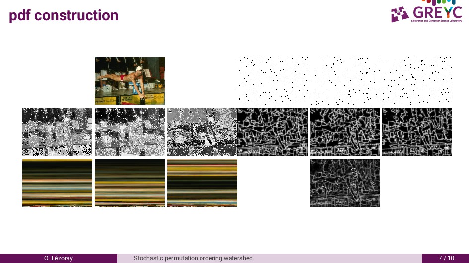
6. pdf construction As the starting vertex is taken at random we can obtain several complete lattices We built M stochastic permutation orderings (Ii, Pi) with i ∈ [1, M] We construct M watersheds from the minima of each ordering WSi(f) = WS(Ii, ∇f) We construct a pdf from the segmentation: pdf(f) = 1 M M i=0 G(WSi(f)) ( ) and combine it with the classical gradient ∇f = pdf(f) + ∇f 2 ( ) This pdf can be used for watershed segmentation from markers O. L´ ezoray Stochastic permutation ordering watershed 6 /
7. pdf construction O. L´ ezoray Stochastic permutation ordering watershed /
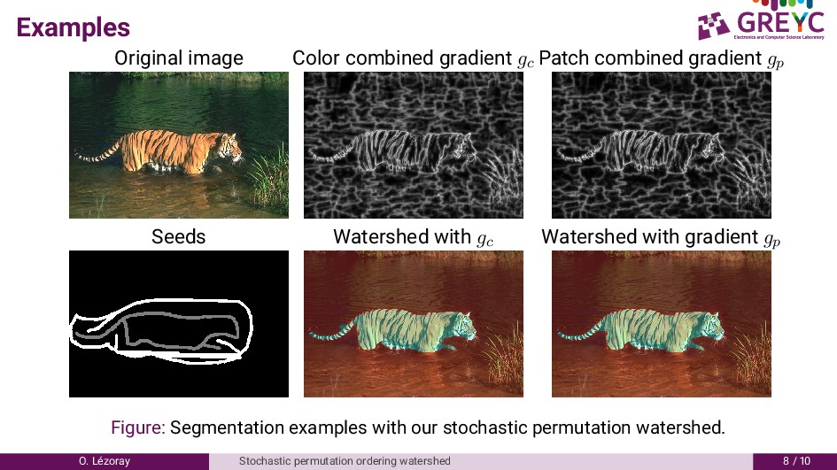
8. Examples Original image Color combined gradient gc Patch combined gradient gp Seeds Watershed with gc Watershed with gradient gp Figure: Segmentation examples with our stochastic permutation watershed. O. L´ ezoray Stochastic permutation ordering watershed 8 /
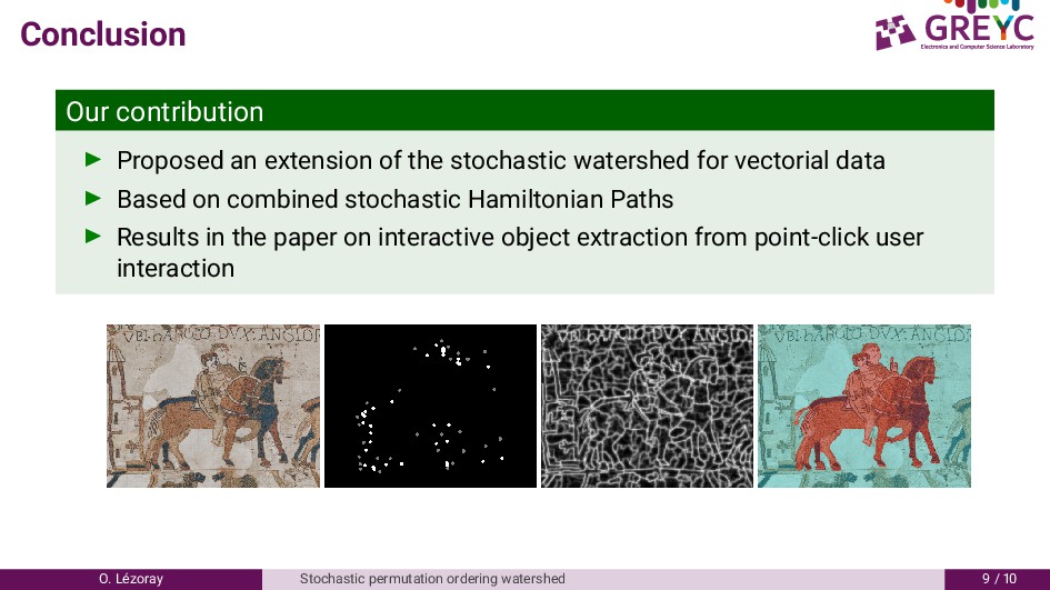
9. Conclusion Our contribution Proposed an extension of the stochastic watershed for vectorial data Based on combined stochastic Hamiltonian Paths Results in the paper on interactive object extraction from point-click user interaction O. L´ ezoray Stochastic permutation ordering watershed /
10. The End Publications available at : https://lezoray.users.greyc.fr O. L´ ezoray Stochastic permutation ordering watershed /