Adaptive Experimental Design for Efficient Average Treatment Effect Estimation and Treatment Choice

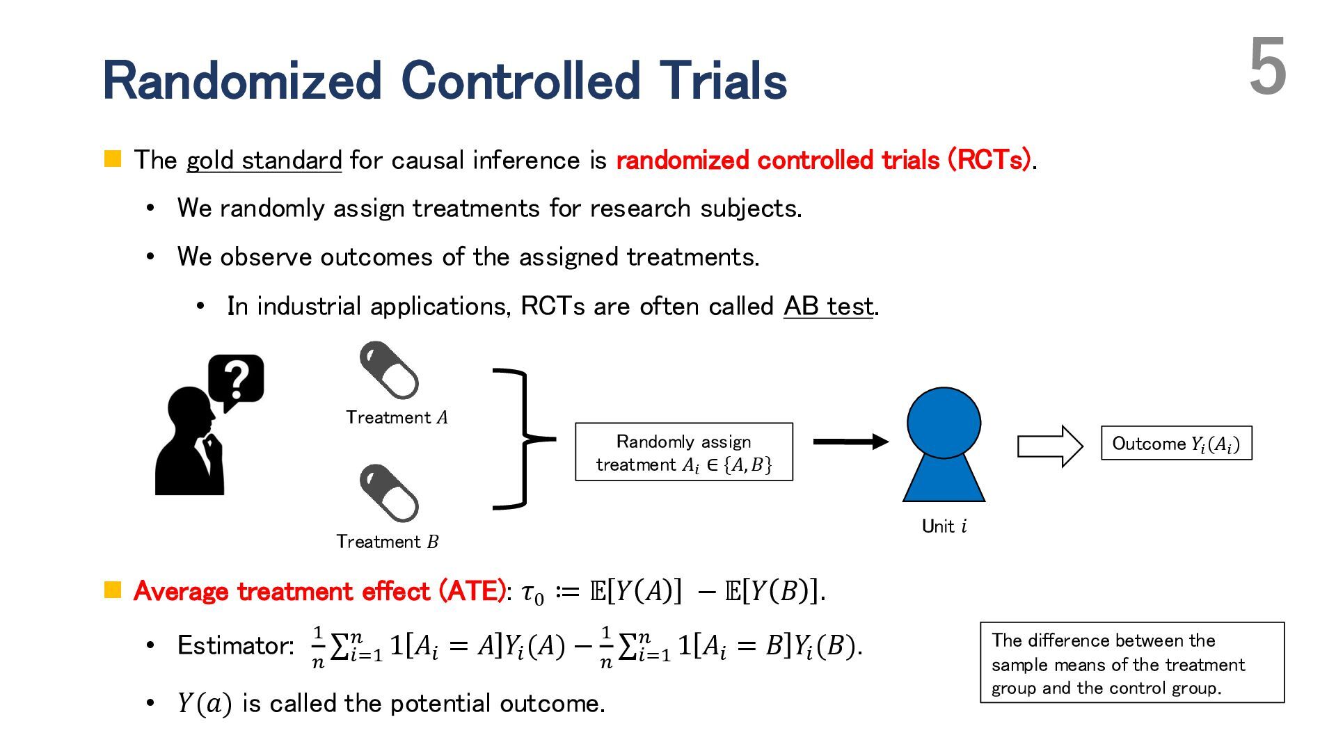
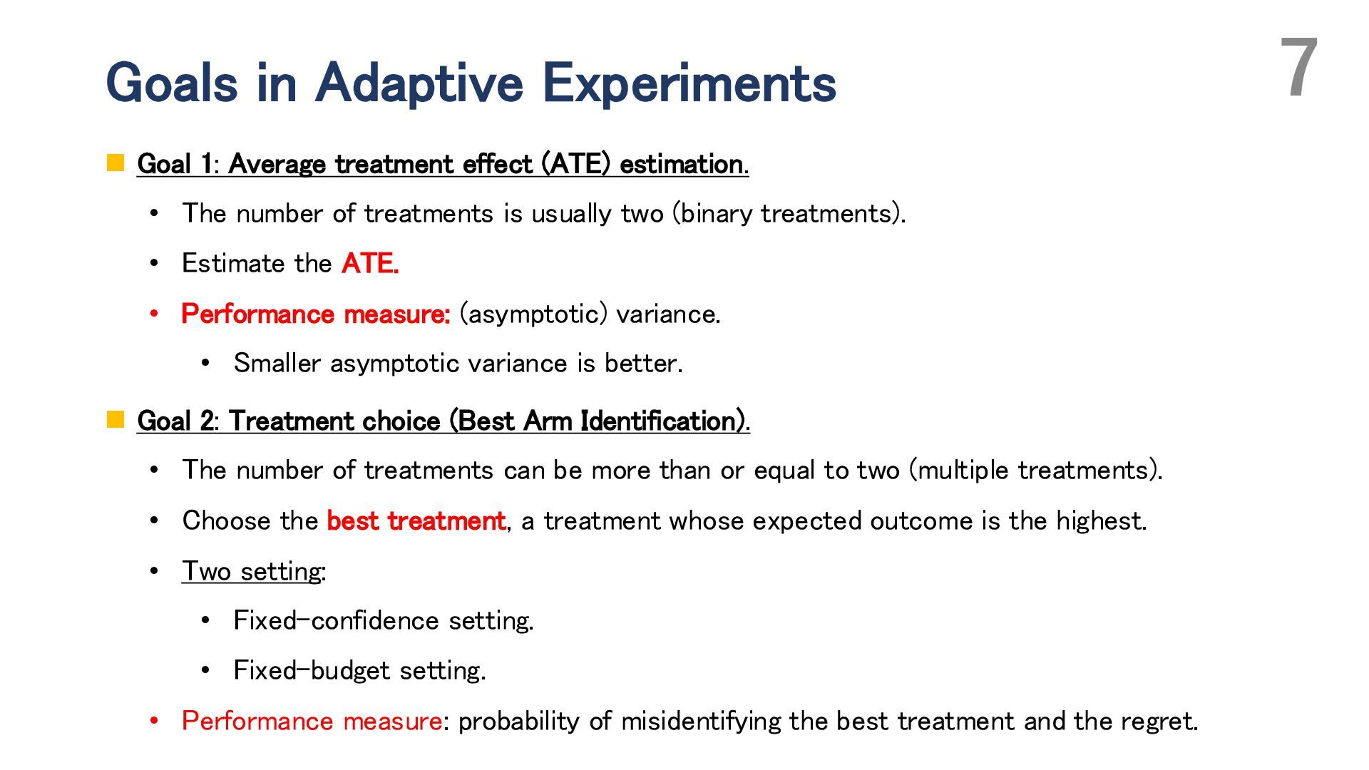
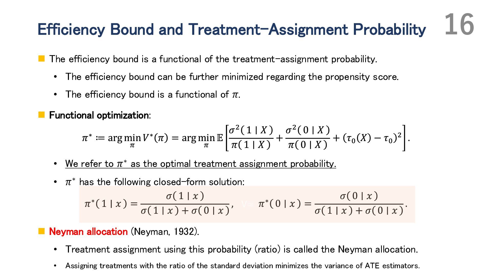
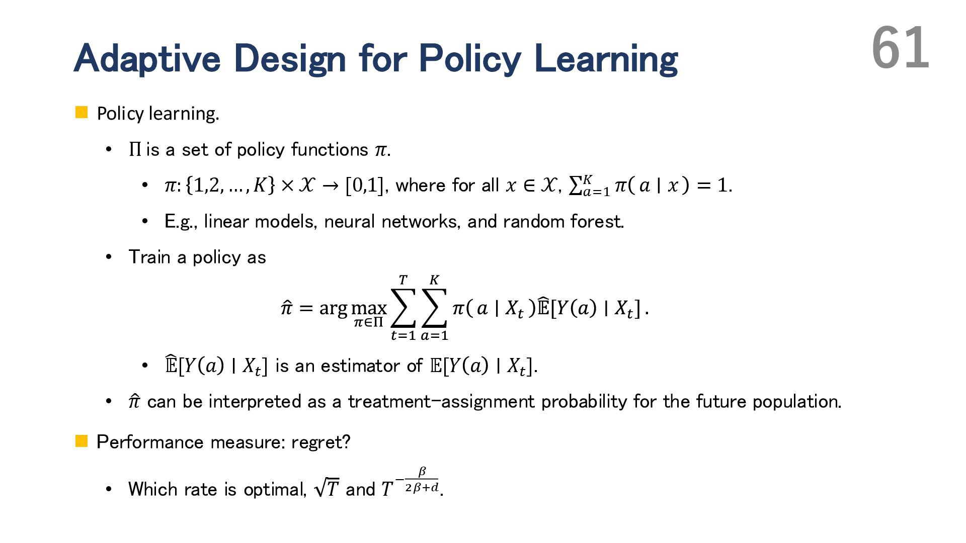
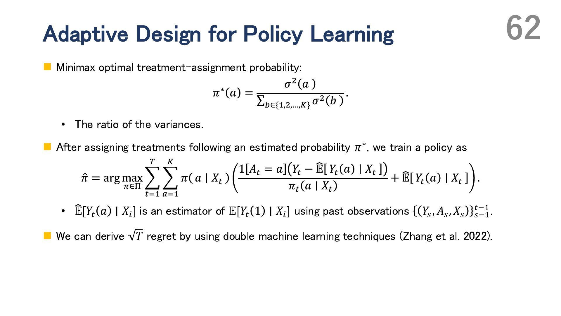
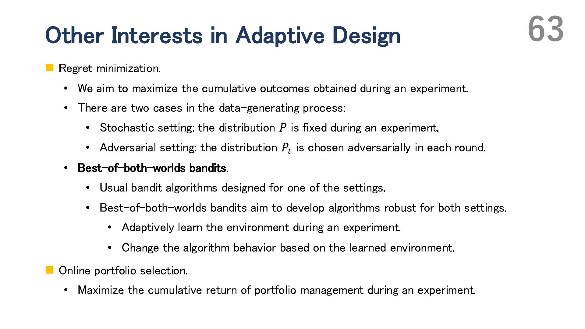
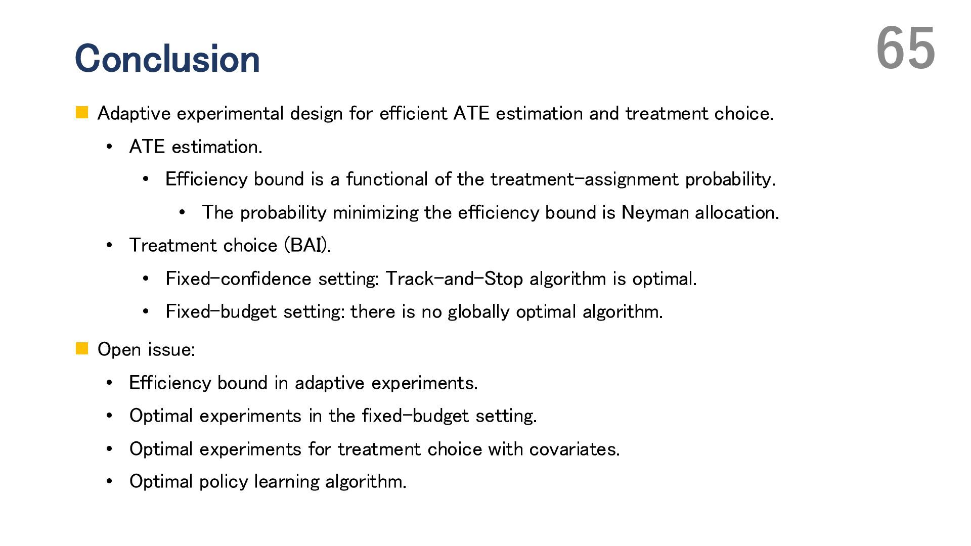
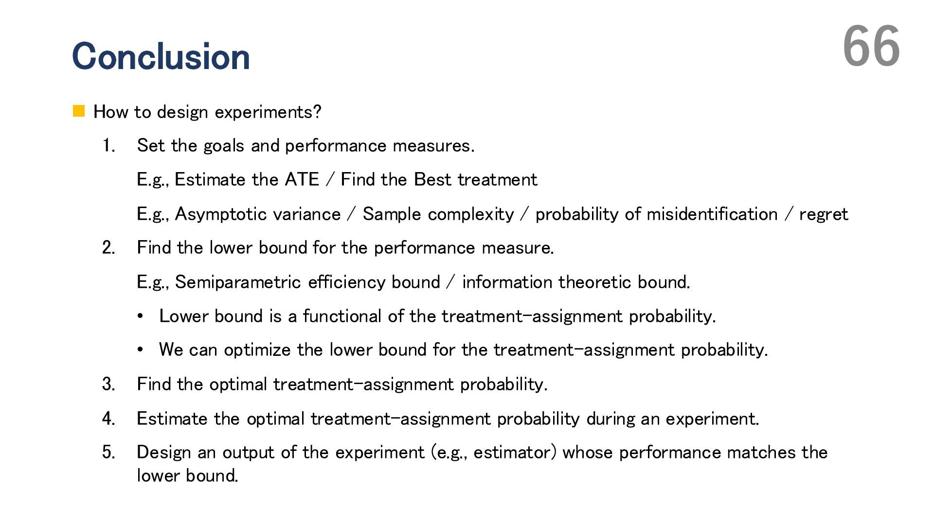
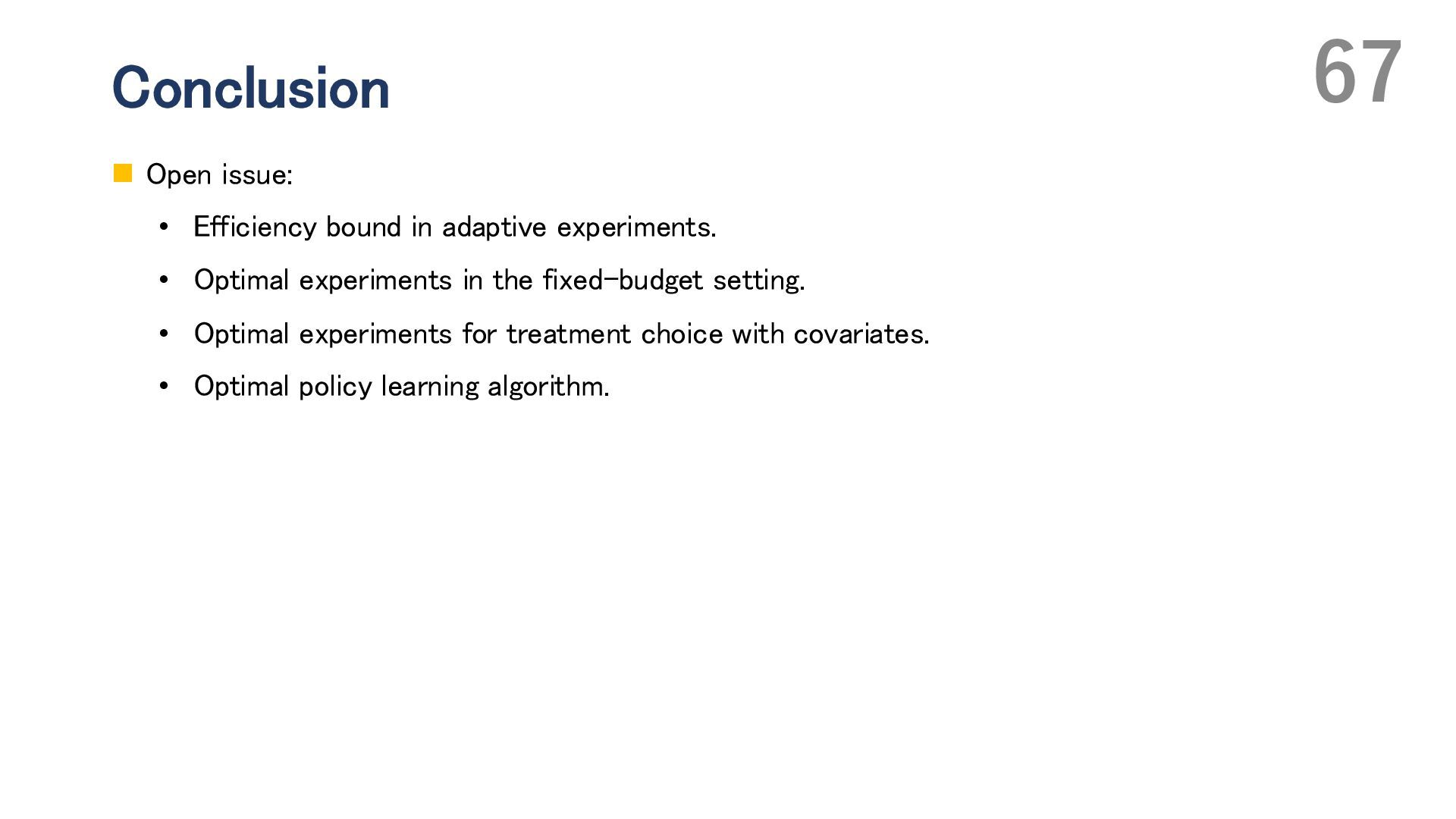
Adaptive experimental design has attracted attention for improving the efficiency of both average treatment effect (ATE) estimation and treatment choice. In such designs, the probability of assigning treatments (i.e., the propensity score) can be updated during the experiment based on previously collected observations. In ATE estimation, the objective is to reduce the estimation error of the ATE, whereas in treatment choice, the goal is to identify the best treatment—the one with the highest expected outcome. While ATE estimation typically involves binary treatments, treatment choice problems often consider multiple treatment options. In this talk, I begin by discussing adaptive experimental design for ATE estimation. I introduce the basic approach based on Neyman allocation, which provides a treatment-assignment probability that minimizes the asymptotic variance of ATE estimators, and then present several extensions, including adaptive optimization of the covariate distribution. Next, I address adaptive experimental design for treatment choice, also known as the best-arm identification problem, and highlight the challenges in developing “optimal” algorithms, especially in the presence of multiple treatments. I propose minimax and Bayes optimal algorithms for treatment choice in the setting without covariates. In particular, I generalize Neyman allocation to construct a minimax optimal algorithm. Finally, I discuss how incorporating covariates can further enhance the efficiency of treatment choice, focusing on conditional treatment choice (policy learning).

Transcript

1. 1 Adaptive Experimental Design for Efficient Average Treatment Effect Estimation and Treatment Choice Brown Bag Seminar Masahiro Kato
2. 2 Treatments and Causal Inference ◼ Treatments: actions whose causal effects (outcomes) we aim to estimate. • E.g., advertisements, marketing approaches, government policies, and medicines. ◼ Causal inference: estimating the causal effects of treatments. Treatment Outcome Researcher Individuals (research subjects, unit) E.g., customers and patients.
3. 3 Causal Effect and Treatment Effect ◼ We are interested in comparison of the outcomes of several treatments. ◼ The difference between the outcomes are called the treatment effect (a causal effect). Treatment 1 Outcome Treatment 2 Outcome Causal effect
4. 4 Counterfactual Inference ◼ For each unit , we can only observe an outcome of one of the treatments. • We cannot observe outcomes of different treatments simultaneously. • E.g., student who receives a scholarship and does not receive the scholarship. • E.g., patient who is given drug A and drug B. • If a unit receives several treatments, we should interpret the combination of the treatments as a new treatment. ◼ Counterfactual property: we cannot observe outcomes of unassigned treatment. Treatment 1 Treatment 2 Treatment 1 Treatment 2 OR × Unit) Unit)
5. 5 Randomized Controlled Trials ◼ The gold standard for causal inference is randomized controlled trials (RCTs). • We randomly assign treatments for research subjects. • We observe outcomes of the assigned treatments. • In industrial applications, RCTs are often called AB test. ◼ Average treatment effect (ATE): 𝜏0 ≔ 𝔼 𝑌 𝐴 − 𝔼 𝑌 𝐵 . • Estimator: 1 𝑛 σ 𝑖=1 𝑛 1 𝐴𝑖 = 𝐴 𝑌𝑖 (𝐴) − 1 𝑛 σ 𝑖=1 𝑛 1 𝐴𝑖 = 𝐵 𝑌𝑖 (𝐵). • 𝑌(𝑎) is called the potential outcome. Treatment 𝐴 Treatment 𝐵 Randomly assign treatment 𝐴𝑖 ∈ {𝐴, 𝐵} Outcome 𝑌𝑖 (𝐴𝑖 ) Unit 𝑖 The difference between the sample means of the treatment group and the control group.
6. 6 Adaptive Experimental Design ◼ RCTs are the gold standard. However, × Costly × Inefficient. → We want to design more efficient experiments (in some sense). ◼ Adaptive experiments: an experiment where we can optimize experiments during the experiments to gain efficiency. • E.g., we can update the treatment-assignment probability during the experiments. ◆Questions in adaptive experimental design: • What treatment-assignment probability and estimators should we use? • What performance measure should we use? Definition of efficiency. • Selection bias occurred by the adaptive optimization • Time series dependency among observations.
7. 7 Goals in Adaptive Experiments ◼ Goal 1: Average treatment effect (ATE) estimation. • The number of treatments is usually two (binary treatments). • Estimate the ATE. • Performance measure: (asymptotic) variance. • Smaller asymptotic variance is better. ◼ Goal 2: Treatment choice (Best Arm Identification). • The number of treatments can be more than or equal to two (multiple treatments). • Choose the best treatment, a treatment whose expected outcome is the highest. • Two setting: • Fixed-confidence setting. • Fixed-budget setting. • Performance measure: probability of misidentifying the best treatment and the regret.
8. 8 Contents ◼ Introduce my series of works on adaptive experimental design. • ATE estimation: • Masahiro Kato, Takuya Ishihara, Junya Honda, and Yusuke Narita. Efficient adaptive experimental design for average treatment effect estimation, 2020. arXiv:2002.05308. • Masahiro Kato, Akihiro Oga, Wataru Komatsubara, and Ryo Inokuchi. Active adaptive experimental design for treatment effect estimation with covariate choice. In International Conference on Machine Learning (ICML), 2024. • Masahiro Kato, Kenichiro McAlinn, and Shota Yasui. The adaptive doubly robust estimator and a paradox concerning logging policy. In International Conference on Neural Information Processing Systems (NeurIPS), 2021. • BAI: • Kaito Ariu, Masahiro Kato, Junpei Komiyama, Kenichiro McAlinn, and Chao Qin. A comment on “adaptive treatment assignment in experiments for policy choice”. Econometrica, 2025. • Masahiro Kato. Generalized Neyman allocation for locally minimax optimal best-arm identification, 2024. arXiv: 2405.19317. • Masahiro Kato and Kaito Ariu. The role of contextual information in best arm identification, 2021 • Junpei Komiyama, Kaito Ariu, Masahiro Kato, and Chao Qin. Rate-optimal Bayesian simple regret in best arm identification. Mathematics of Operations Research, 2023. • Masahiro Kato, Kyohei Okumura, Takuya Ishihara, and Toru Kitagawa. Adaptive experimental design for policy learning, 2024. arXiv: 2401.03756.
9. 9 Adaptive Experimental Design for Efficient Average Treatment Effect Estimation • Masahiro Kato, Takuya Ishihara, Junya Honda, and Yusuke Narita. Efficient adaptive experimental design for average treatment effect estimation, 2020. arXiv:2002.05308. Updated 2025. • Masahiro Kato, Kenichiro McAlinn, and Shota Yasui. The adaptive doubly robust estimator and a paradox concerning logging policy. In International Conference on Neural Information Processing Systems (NeurIPS), 2021. • Masahiro Kato, Akihiro Oga, Wataru Komatsubara, and Ryo Inokuchi. Active adaptive experimental design for treatment effect estimation with covariate choice. In International Conference on Machine Learning (ICML), 2024a.
10. 10 Problem Formulation ◼ Two treatments indexed by 1 and 0 and 𝑇 units indexed by 1,2, … , 𝑇. • For each 𝑡 = 1,2, …, we can assign one of the treatments, 1 and 0. ◼ Potential outcome 𝑌𝑡 1 , 𝑌𝑡 (0) ∈ ℝ． ◼ 𝑑-dimensional covariates 𝑋𝑡 ∈ 𝒳 ⊂ ℝ𝑑. • E.g., Characteristics of each unit 𝑡. E.g., Age, occupation, etc. ◼ 𝑌𝑡 1 , 𝑌𝑡 (0), 𝑋𝑡 jointly follows a distribution 𝑃0 . Treatment 1 Unit 𝑡 with Covariates 𝑋𝑡 E.g., Age, occupation, etc. Treatment 0 Outcome 𝑌(1). Outcome 𝑌(0).
11. 11 Problem Formulation ➢ We consider a decision-maker who conducts the following adaptive experiment. ◼ Adaptive experimental design with 𝑇 rounds (𝑇 units): • Experimental units sequentially appear in each round 𝑡 = 1,2, … , 𝑇. • Using the covariates 𝑋𝑡 and past observations, the decision-maker assigns a treatment 𝐴𝑡 ∈ {1, 0}. • The decision-maker observes the outcome 𝑌𝑡 = 1 𝐴𝑡 = 1 𝑌𝑡 1 + 1 𝐴𝑡 = 0 𝑌𝑡 (0). • At the end, the decision-maker estimates the ATE 𝜏 = 𝔼 𝑌 1 − 𝔼 𝑌 0 . Round 𝒕 Unit 𝑡 with Covariates 𝑋𝑡 Treatment 𝐴𝑡 Covariate 𝑋𝑡 Outcome 𝑌𝑡 After round 𝑻 • Estimate the ATE.
12. 12 Problem Formulation ◼ Formal procedure: 1. Treatment-assignment phase: in each round 𝑡 = 1,2, … , 𝑇: • (𝑌𝑡 1 , 𝑌𝑡 0 , 𝑋𝑡 ) is generated from 𝑃0 . • Observes covariates 𝑋𝑡 . • Assigns treatment 𝐴𝑡 ∈ {1,0} based on 𝑋𝑠 , 𝐴𝑠 , 𝑌𝑠 𝑠=1 𝑡−1 and 𝑋𝑡 . • Observes the outcome 𝑌𝑡 = 1 𝐴𝑡 = 1 𝑌𝑡 1 + 1 𝐴𝑡 = 0 𝑌𝑡 0 . 2. Decision-making phase: at the end of the experiment (after observing 𝑋𝑡 , 𝐴𝑡 , 𝑌𝑡 𝑡=1 𝑇 ). • Estimate the ATE 𝜏 = 𝔼 𝑌 1 − 𝔼 𝑌 0 . V≈
13. 13 Problem Formulation ◼ We can optimize a treatment-assignment probability and an estimator. ① A treatment-assignment probability 𝜋𝑡 𝐴𝑡 𝑋𝑖 = 𝑃 𝐴𝑡 𝑋𝑡 , ℱ𝑡 in the treatment-assignment phase. • ℱ𝑡 = 𝑋1 , 𝐴1 , 𝑌1 , … , 𝑋𝑡−1 𝐴𝑡−1 𝑌𝑡−1 is the set of past observations. ② An ATE estimator Ƹ 𝜏𝑛 in the decision-making phase. Algorithm = Treatment-assignment probability + ATE estimator. ◼ How to decide the treatment-assignment probability and the ATE estimator? • Set an optimality criterion. • Find the optimal treatment-assignment probability. • Construct an estimator whose performance attains the optimality. V≈
14. 14 Performance Measure ➢ What treatment-assignment probability 𝜋𝑡 and estimator Ƹ 𝜏𝑛 should we use? ◼ We aim to construct an asymptotically normal estimator Ƹ 𝜏𝑛 with a smaller asymptotic variance: 𝑇 Ƹ 𝜏𝑇 − 𝜏 →𝑑 𝒩 0, 𝑉 as 𝑛 → ∞. • Smaller asymptotic variance? • Theoretically best asymptotic variance is given by the semiparametric efficiency bound. • Lower bound for the asymptotic variance of regular estimators. • Cf. Cramer-Rao lower bound. • Estimators whose asymptotic variance matches the efficiency bound is called efficient. V≈ Regular estimators Asymptotic variance Efficiency bound Efficient estimator
15. 15 Efficiency Bound ◼ Consider the following data-generating process (DGP_: 𝑋, 𝐴, 𝑌 ∼ 𝑝 𝑥, 𝑎, 𝑦 ≔ 𝑞 𝑥 𝜋 1 𝑥 𝜁1 𝑦 𝑥 1 𝑎=1 𝜋 0 𝑥 𝜁0 𝑦 𝑥 1 𝑎=0 . • 𝜋(𝑎 ∣ 𝑥): a treatment-assignment probability (propensity score). • The decision-makers can optimize 𝜋 by themselves. ◼ Efficiency bound for ATE estimation (Hahn, 1998): • If observations are i.i.d. under the above DGP, the asymptotic variance of any regular estimators is lower bounded by 𝑉∗ 𝜋 ≔ 𝔼 𝜎2 1 𝑋 𝜋 1 𝑋 + 𝜎2 0 𝑋 𝜋 0 𝑋 + 𝜏 𝑋 − 𝜏 2 . • 𝜏 𝑥 is the conditional ATE defined as 𝜏 𝑋 ≔ 𝔼[𝑌 1 ∣ 𝑋] − 𝔼[𝑌 0 ∣ 𝑋]. • 𝜎2(𝑎 ∣ 𝑋) ≔ 𝑉𝑎𝑟 𝑌 𝑎 𝑋 .is the conditional variance of the outcome 𝑌(𝑎). ◼ We simply consider the efficiency bound under a fixed treatment-assignment probability 𝜋. • This approach is same as Hahn, Hirano, and Karlan (2011). • Lower bounds have several variants. E.g., Kallus, Saito, and Uehara (2021); Li et al. (2023); Rafi (2023). V≈ V≈
16. 16 Efficiency Bound and Treatment-Assignment Probability ◼ The efficiency bound is a functional of the treatment-assignment probability. • The efficiency bound can be further minimized regarding the propensity score. • The efficiency bound is a functional of 𝜋. ◼ Functional optimization: 𝜋∗ ≔ arg min 𝜋 𝑉∗ 𝜋 = arg min 𝜋 𝔼 𝜎2 1 𝑋 𝜋 1 𝑋 + 𝜎2 0 𝑋 𝜋 0 𝑋 + 𝜏0 𝑋 − 𝜏0 2 . • We refer to 𝜋∗ as the optimal treatment assignment probability. • 𝜋∗ has the following closed-form solution: 𝜋∗ 1 𝑥 = 𝜎 1 𝑥 𝜎 1 𝑥 + 𝜎 0 𝑥 , 𝜋∗ 0 𝑥 = 𝜎 0 𝑥 𝜎 1 𝑥 + 𝜎 0 𝑥 . ◼ Neyman allocation (Neyman, 1932). • Treatment assignment using this probability (ratio) is called the Neyman allocation. • Assigning treatments with the ratio of the standard deviation minimizes the variance of ATE estimators. V≈
17. 17 Neyman Allocation ◼ Neyman allocation (Neyman, 1932). • Treatment assignment using the optimal treatment-assignment probability (ratio) is called the Neyman allocation. 𝜋∗ 1 𝑥 = 𝜎 1 𝑥 𝜎 1 𝑥 + 𝜎 0 𝑥 , 𝜋∗ 0 𝑥 = 𝜎 0 𝑥 𝜎 1 𝑥 + 𝜎 0 𝑥 . • Assigning treatments with the ratio of the standard deviation minimizes the variance of ATE estimators. ◼ The variances (standard deviations) are usually unknown. • If they are unknown, the Neyman allocation is infeasible. ◼ In adaptive experiment, we aim to estimate the variance during the experiment. • During an experiment, we simultaneously estimate the variance and assign treatment following an estimated treatment-assignment probability.
18. 18 Batch and Sequential Design ◼ In adaptive experimental design, there are two types design: • Batch design: update the treatment-assignment probability only at a predetermined rounds. • E.g., Update the probability only at round 100, 200, 300, ... • E.g., Two-stage experiment. • Split 1000 rounds into two stages: the first 300 rounds and the next 700 rounds. • The first stage is pilot phase: we estimate parameters, such as variances. • In the next stage, we assign treatments following the probability estimated in the first stage. • Sequential design: update the treatment-assignment probability at every rounds. ✓ Batch design can be considered a restricted case for sequential design. 𝑇 𝑡 = 1 Sequential design Batch design
19. 19 Batch Design ⚫ Hahn, Hirano, and Karlan. “Adaptive Experimental Design Using the Propensity Score.” Journal of Business and Economic Statistics 2011. • Two-stage batch experiment. • In the first stage, they estimate the conditional variance 𝜎2 𝑎 𝑋 . • In the second stage, they assign treatments with the optimal probability: 𝜋∗ 1 𝑥 = 𝜎 1 𝑥 𝜎 1 𝑥 + 𝜎 0 𝑥 , 𝜋∗ 0 𝑥 = 𝜎 0 𝑥 𝜎 1 𝑥 + 𝜎 0 𝑥 . ➢ Issues: • They only consider discrete covariates. → How we deal with continuous covariates? • Can we improve the estimation of the treatment-assignment probability by updating it more frequently?
20. 20 Sequential Design ⚫ Kato, Ishihara, Honda, and Narita.“Efficient Average Treatment Effect Estimation via Adaptive Experiments.” 2020 arXiv. ◼ Efficient sequential ATE estimation: 1. Treatment-assignment phase: in each round 𝑡 = 1,2, … , 𝑇: I. Observe 𝑋𝑡 . II. Construct estimator ො 𝜎𝑡 2(𝑎 ∣ 𝑋𝑡 ) of 𝜎2(𝑎 ∣ 𝑋𝑡 ) using past observations 𝑌𝑠 , 𝐴𝑠 , 𝑋𝑠 𝑠=1 𝑡−1. III. Assign 𝐴𝑡 ∼ 𝜋𝑡 𝑎 𝑋𝑡 = ෝ 𝜎𝑡(1∣𝑋𝑡) ෝ 𝜎𝑡(1∣𝑋𝑡)+ ෝ 𝜎𝑡(0∣𝑋𝑡) . 2. Decision-making phase: at the end of the experiment: • Adaptive Augmented Inverse Probability Weighting (A2IPW) estimator: Ƹ 𝜏𝑇 A2IPW = 1 𝑇 ෍ 𝑡∈[𝑇] 1 𝐴𝑡 = 1 𝑌𝑡 − ෡ 𝔼 𝑌𝑡 1 𝑋𝑡 𝜋𝑡 1 ∣ 𝑋𝑡 − 1 𝐴𝑡 = 0 𝑌𝑡 − ෡ 𝔼 𝑌𝑡 0 𝑋𝑡 𝜋𝑡 0 ∣ 𝑋𝑡 + ෡ 𝔼 𝑌𝑡 1 𝑋𝑖 − ෡ 𝔼 𝑌𝑡 0 𝑋𝑖 . • ෡ 𝔼[𝑌𝑡 𝑎 ∣ 𝑋𝑖 ] is an estimator of 𝔼[𝑌𝑡 1 ∣ 𝑋𝑖 ] using past observations 𝑌𝑠 , 𝐴𝑠 , 𝑋𝑠 𝑠=1 𝑡−1. V≈
21. 21 Asymptotic Normality and Efficiency ◼ Rewrite the A2IPW estimator as Ƹ 𝜏𝑇 A2IPW = 1 𝑇 ෍ 𝑡=1 𝑇 𝜓𝑡 . • 𝜓𝑡 ≔ 1 𝐴𝑡=1 𝑌𝑡−෡ 𝔼 𝑌𝑡 1 𝑋𝑖 𝜋𝑡 1∣𝑋𝑡 − 1 𝐴𝑡=0 𝑌𝑡−෡ 𝔼 𝑌𝑡 0 𝑋𝑖 𝜋𝑡 0∣𝑋𝑡 + ෡ 𝔼 𝑌𝑡 1 𝑋𝑖 − ෡ 𝔼 𝑌𝑡 0 𝑋𝑖 . ◼ 𝜓𝑡 𝑡=1 𝑇 is a martingale difference sequence. • Under suitable conditions, we can apply the martingale central limit theorem. • We can address the sample dependency problem occurred by the adaptive sampling. • m (Asymptotic normality of the A2IPW estimator): • 𝜋𝑡 𝑎 𝑋 − 𝜋∗ 𝑎 𝑋 → 0 and ෡ 𝔼[𝑌𝑡 𝑎 ∣ 𝑋] → 𝔼[𝑌 𝑎 ∣ 𝑋] as 𝑡 → ∞ almost surely. • Then, the following holds: 𝑇 Ƹ 𝜏𝑇 A2IPW − 𝜏 → 𝑑 𝒩 0, 𝑉 𝜋∗ 𝑎𝑠 𝑇 → ∞ Theorem (Asymptotic normality of the A2IPW estimator) V≈ V≈
22. 22 Double Machine Learning ◼ The proof of the asymptotic normality is related to that in double machine learning (Chernozhukov et al., 2018). ➢ Kato, Yasui, and McAlinn. “The Adaptive Doubly Robust Estimator for Policy Evaluation in Adaptive Experiments and a Paradox Concerning Logging Policy.” NeurIPS (2021). ◼ We can replace the true probability 𝜋𝑡 with its estimator even if we know 𝜋𝑡 . • Since 𝜋𝑡 can be volatile, replacing it with its estimator can stabilize the performance. ◼ The asymptotic property does not change. • The use of past observations is a variant of sample splitting, recently called cross fitting. • See Klaassen, 1987, van der Laan (2008), and Chernozhukov et al. (2018). • Kato, Yasui, and McAlinn (2021) refers to the sample splitting as adaptive fitting (Figure 1).
23. 23 Hypothesis Testing ◼ Consider the following null hypothesis and alternative hypothesis: 𝐻0 : 𝜏 = 0, 𝐻1 : 𝜏 ≠ 0. ◼ There are two types of hypothesis testing. 1. Single-stage testing. • At the end of the fixed round 𝑇, we estimate the ATE and conduct hypothesis testing. 2. Sequential testing. • We can conduct hypothesis testing at any round 𝑡 and can stop the experiment. • Sequential testing allows us to conduct early stopping. • If the null 𝐻0 can be rejected easily, we stop the experiment as soon as possible. • Our study develops anytime valid confidence interval for sequential testing. V≈
24. 24 Efficiency Gain  How the adaptive sampling improves the efficiency? ◼ Sample size computation in the single-stage hypothesis testing with 𝐻0 : 𝜏 = 0, 𝐻1 : 𝜏 = Δ. • Treatment-assignment probability 𝜋. An effect size Δ ≠ 0. • To achieve a power 𝛽 with controlling Type I error at 𝛼, we need samples at least 𝑇∗ 𝜋 ≔ 𝑉∗ 𝜋 Δ2 𝑧1 −𝛼/2 − 𝑧𝛽 2 • 𝑧𝑤 is the 𝑤 quantile of the standard normal distribution. ◼ Sample size comparison. • Setting: 𝑋 ∈ Uniform[0, 1], 𝜎2 1 𝑋 = 𝑋2, 𝜎2 0 𝑋 = 0.1, Δ = 0.1, 𝛼 = 𝛽 = 0.05, 𝜏 𝑋 = 𝜏 = Δ. • RCT (𝜋 1 𝑋 = 𝜋 0 𝑋 = 1/2): 𝑇∗ 𝜋 ≈ 1300. • Neyman allocation: 𝑇∗ 𝜋 ≈ 970. • Another case: 𝜎2 1 𝑋 = (2𝑋)2, 𝜎2 0 𝑋 = 0.1. RCT: 𝑇∗ 𝜋 ≈ 3700. Neyman allocation: 𝑇∗ 𝜋 ≈ 2600. Reduce 330 samples. V≈
25. 25 Covariate Distribution Optimization ◼ Can we further reduce the sample size (gain efficiency)? → Active adaptive experimental design: select the experimental units. • Optimize the covariate density 𝑝𝑡 (𝑥) of 𝑋𝑡 as well as the treatment probability 𝜋𝑡 . ➢ Kato, Oga, Komatsubara, and Inokuchi. “Active Adaptive Experimental Design for Treatment Effect Estimation with Covariate Choices.” ICML (2024) ◼ Recall that the ATE is defined as 𝜏 ≔ ∫ 𝑦 1 − 𝑦 0 𝜁 𝑦 1 , 𝑦 0 𝑥 𝑞 𝑥 𝑑𝑦 1 𝑑𝑦 0 𝑑𝑥. ◼ Target covariate density: 𝑞(𝑥). ◼ Sample covariate density at round 𝑡: 𝑝𝑡 (𝑥). • Covariate density can be also optimized during an experiment. • Covariate density represents the histogram of the characteristics of experimental units. • C.f., covariate shift (Shimodaira 2000): evaluation density 𝑞0 (𝑥) is different from observation density 𝑝𝑡 (𝑥).
26. 26 Covariate Distribution Optimization ◼ Active adaptive experiment: In each round 𝑡 ∈ [𝑇], ① We obtain experimental unit with covariates 𝑋𝑡 generated from optimized 𝑝𝑡 (𝑥). ② Observe 𝑋𝑡 and assign treatment 𝐴𝑡 with probability 𝜋𝑡 (𝐴𝑡 ∣ 𝑋𝑡 ). ③ Observe the outcome 𝑌𝑡 = 𝑌(𝐴𝑡 ). • Estimate the ATE or choose a treatment arm using 𝑋𝑡 , 𝐴𝑡 , 𝑌𝑡 𝑡=1 𝑇 . At the end of the experiment, we estimate the ATE by Ƹ 𝜏𝑇 . We can optimize them. ① Gather experimental units ③ Observe the outcome ② Treatment The pool of Experimental units Target population Decision-maker Experimental unit
27. 27 Covariate Distribution Optimization ◼ Given a covariate density 𝑝(𝑥) and a treatment-assignment probability 𝜋(𝑎 ∣ 𝑥), consider the DGP: 𝑋, 𝐴, 𝑌 ∼ 𝑝 𝑥, 𝑎, 𝑦 ≔ 𝑝 𝑥 𝜋 1 𝑥 𝜁 𝑦 1 𝑥 1 𝑑=1 𝜋 0 𝑥 𝜁 𝑦 0 𝑥 1 𝑑=0 . ◼ The efficiency bound for the ATE defined over 𝑋 generated from 𝑞0 (𝑥) is given as 𝑉∗ 𝑝, 𝜋 ≔ න 𝜎2 1 𝑥 𝜋 1 𝑥 + 𝜎2 0 𝑥 𝜋 0 𝑥 𝑞 𝑥 𝑝 𝑥 𝑞 𝑥 𝜁 𝑦 1 , 𝑦 0 𝑥 𝑑𝑦 1 𝑑𝑦 0 𝑑𝑥. • The efficiency bound is a functional of 𝑝 and 𝜋. • Denote the minimizer of 𝑉∗(𝑝, 𝜋) as (𝑝∗, 𝜋∗) ≔ arg min 𝑝,𝜋 𝑉∗ 𝑝, 𝜋 . ◼ Their closed-form solutions exist as follows: 𝑝∗ 𝑥 = 𝜎(1 ∣ 𝑥) + 𝜎(0 ∣ 𝑥) ∫ 𝜎(1 ∣ 𝑥) + 𝜎(0 ∣ 𝑥) 𝑞 𝑥 𝑑𝑥 , 𝜋∗ 𝑎 𝑥 = 𝜎(𝑎 ∣ 𝑥) 𝜎(1 ∣ 𝑥) + 𝜎(0 ∣ 𝑥) . • 𝜋∗ is the same as the one in the case with the fixed covariate density (Neyman allocation). V≈ V≈
28. 28 Covariate Distribution Optimization ◼ Optimal treatment-assignment probability: 𝜋∗ 𝑎 𝑋 = 𝜎(𝑎∣𝑋) 𝜎(1∣𝑋)+𝜎(0∣𝑋) . • Neyman allocation. ◼ Optimal covariate density: 𝑝∗ 𝑥 = 𝜎(1∣𝑥)+𝜎(0∣𝑥) ∫ 𝜎(1∣𝑥)+𝜎(0∣𝑥) 𝑞 𝑥 𝑑𝑥 . • We sample experimental units with higher variances. ✓ 分布𝑞∗上の平均処置効果に関心があっても，分散を小さくできる密度は𝑝∗(𝑥) ≠ 𝑞(𝑥)． ◼ Estimate the ATE using the following Importance-Weighting A2IPW (IWA2IPW)estimator: Ƹ 𝜏𝑇 IWA2IPW = 1 𝑇 ෍ 𝑡∈[𝑇] 1 𝐴𝑡 = 1 𝑌𝑡 − ෡ 𝔼[𝑌𝑡 1 ∣ 𝑋] 𝜋𝑡 1 ∣ 𝑋𝑡 − 1 𝐴𝑡 = 0 𝑌𝑡 − ෡ 𝔼[𝑌𝑡 0 ∣ 𝑋] 𝜋𝑡 0 ∣ 𝑋𝑡 𝑞 (𝑋𝑡 ) 𝑝𝑡 (𝑋𝑡 ) + න ෡ 𝔼[𝑌𝑡 1 ∣ 𝑋] − ෡ 𝔼[𝑌𝑡 0 ∣ 𝑋] 𝑞0 𝑥 𝑑𝑥 . 𝒒(𝒙)
29. 29 Adaptive Experimental Design for Treatment Choice • Kaito Ariu, Masahiro Kato, Junpei Komiyama, Kenichiro McAlinn, and Chao Qin. A comment on “adaptive treatment assignment in experiments for policy choice.” 2021. • Masahiro Kato. Generalized Neyman allocation for locally minimax optimal best-arm identification, 2024. arXiv: 2405.19317. • Masahiro Kato. Locally optimal fixed-budget best arm identification in two-armed gaussian bandits with unknown variances, 2024. arXIV: 2312.12741. • Masahiro Kato and Kaito Ariu. The role of contextual information in best arm identification, 2021. • Masahiro Kato, Kyohei Okumura, Takuya Ishihara, and Toru Kitagawa. Adaptive experimental design for policy learning, 2024b. arXiv: 2401.03756. • Junpei Komiyama, Kaito Ariu, Masahiro Kato, and Chao Qin. Rate-optimal bayesian simple regret in best arm identification. Mathematics of Operations Research, 2023
30. 30 From ATE Estimation to Treatment Choice ◼ From ATE estimation to decision-making (treatment choice). • We discussed how we estimate the ATE (causal effect). • Consider a decision-making about the choice of actions based on the causal inference. • Such a decision-making problem is called the treatment choice problem. ◼ Treatment choice via adaptive experiments is called best-arm identification (BAI). • Treatment choice problem has been investigated in various areas, including operations research and economics (Manski, 2004). • The treatment choice problem with adaptive experimental design is called the BAI problem. Gathering data Parameter estimation Decision-making ATE estimation Treatment choice
31. 31 Problem Formulation ◼ 𝐾 treatments indexed by 1,2, … 𝐾． • Also referred to as treatment arms or arms. ◼ Potential outcome 𝑌(𝑎) ∈ ℝ． ◼ (Optional) 𝑑-dimensional covariates 𝑋 ∈ ℝ𝑑. • The use of covariates is a difficult problem in treatment choice, unlike ATE estimation. ◼ 𝑌 1 , 𝑌 2 , … , 𝑌 𝐾 , 𝑋 jointly follows a distribution 𝑃0 . ◼ Goal：Find the following best treatment arm efficiently for some performance metric: 𝑎𝑃0 ∗ ≔ arg max 𝑎∈ 1,2,…,𝐾 𝔼𝑃0 [𝑌(𝑎)] . • In each round 𝑡, we assign treatment 𝐴𝑡 ∈ 1,2, … , 𝐾 . • At the end of the experiment, we estimate the best arm 𝑎𝑃0 ∗ . • We denote the estimator by ො 𝑎𝑇 ∈ 1,2, … , 𝐾 .
32. 32 Problem Formulation ◼ Adaptive experimental design with 𝑇 rounds (BAI): • Treatment-assignment phase: in each round 𝑡 = 1,2, … , 𝑇: • (If possible) Observe covariates 𝑋𝑡 . • Assign treatment 𝐴𝑡 ∈ 1,2, … , 𝐾 using 𝑋𝑠 , 𝐴𝑠 , 𝑌𝑠 𝑠=1 𝑡−1. • Observe the outcome 𝑌𝑡 = σ 𝑎∈ 1,2,…,𝐾 1 𝐴𝑡 = 𝑎 𝑌𝑡 (𝑎). • Decision-making phase: at the end of the experiment (after observing 𝑋𝑡 , 𝐴𝑡 , 𝑌𝑡 𝑡=1 𝑇 ). • Obtain an estimator ො 𝑎𝑇 of the the best treatment arm using 𝑋𝑡 , 𝐴𝑡 , 𝑌𝑡 𝑡=1 𝑇 . Round 𝒕 Unit 𝑡 with Covariates 𝑋𝑡 Treatment 𝐴𝑡 Covariate 𝑋𝑡 Outcome 𝑌𝑡 After round 𝑻 Choose the best treatment.
33. 33 Problem Formulation ◼ BAI has two formulations: fixed-confidence setting and fixed budget setting. • Fixed-confidence setting: Continue until the probability ℙ𝑃 ො 𝑎𝑡 ≠ 𝑎𝑃 ∗ satisfies a criterion. • The sample size 𝑇 is a random variable, not predetermined. • Given a threshold 𝛿 ∈ (0,1), in a round 𝑡, if ℙ𝑃 ො 𝑎𝑡 ≠ 𝑎𝑃 ∗ ≤ 𝛿 is satisfied, then a decision-maker stop the experiment and return an estimated best treatment. • Goal: minimize 𝔼𝑃0 [𝑇], while satisfying ℙ𝑃 ො 𝑎𝑇 ≠ 𝑎𝑃 ∗ ≤ 𝛿. • Fixed-budget setting: Continue for 𝑇 rounds and stop at the end of the 𝑇 round. • The sample size 𝑇 is given and fixed. • After round 𝑇, a decision-maker returns an estimated best treatment. • Goal: minimize ℙ𝑃 ො 𝑎𝑇 ≠ 𝑎𝑃 ∗ . 𝑇: given and fixed. Fixed-confidence setting Fixed-budget setting × △ △ △ △ △ △ △ △ △ △ 𝑇: random and not fixed. If ℙ𝑃 ො 𝑎𝑡 ≠ 𝑎𝑃 ∗ ≤ 𝛿 is satisfied, we stop the experiment. 𝑡
34. 34 Performance Measures ◼ Two important notions: probability of misidentification and expected simple regret. • Probability of misidentification: ℙ𝑃0 ො 𝑎𝑇 ≠ 𝑎𝑃0 ∗ . • Expected simple regret: Regret𝑃0 ≔ 𝔼𝑃0 𝑌 𝑎𝑃0 ∗ − 𝑌 ො 𝑎𝑇 . • Relative welfare loss when we recommend a suboptimal treatment arm instead of the best treatment. • The simple regret has the following equivalent expression: Regret𝑃0 = 𝔼𝑃0 𝑌 𝑎𝑃0 ∗ − 𝔼𝑃0 𝑌 ො 𝑎𝑇 = ෍ 𝑏≠𝑎𝑃0 ∗ 𝔼𝑃0 𝑌 𝑎𝑃0 ∗ − 𝔼𝑃0 𝑌 𝑏 ℙ𝑃0 (ො 𝑎𝑇 ≠ 𝑎𝑃0 ∗ ). • This regret is also called out-of-sample regret. • C.f., In-sample regret (regret minimization). • Maximize the cumulative outcomes obtained during the experiment. ◼ We use different performance measures for fixed-confidence and fixed-budget settings.
35. 35 Performance Measures ◼ Fixed-confidence setting: • We continue an experiment until the probability of misidentification ℙ𝑃0 ො 𝑎𝑻 ≠ 𝑎𝑃0 ∗ lowers the predefined confidence level 𝛿 ∈ {1, 0}. • We aim to design an adaptive experiment that stops with the smallest units (as early as possible). • Performance measure: • Sample complexity (the expected sample size) ：𝔼 𝑇 . • The number of rounds is random variable (stopping time). • We can stop when ℙ𝑃0 ො 𝑎𝑻 ≠ 𝑎𝑃0 ∗ ≤ 𝛿.
36. 36 Performance Measures ◼ Fixed-budget setting: • The sample size 𝑇 is given and fixed. • We continue an experiment until round 𝑇 finishes. • We aim to design an adaptive experiment that stops with the smallest units (as early as possible). • Performance measure: • Probability of misidentification: ℙ𝑃0 ො 𝑎𝑇 ≠ 𝑎∗ 𝑃0 . • Expected simple regret: Regret𝑃 ≔ 𝔼𝑃0 𝑌 𝑎𝑃0 ∗ − 𝑌 ො 𝑎𝑇 .
37. 37 Multi-Armed Bandit Problem. ◼ BAI = adaptive experimental design for treatment choice. • An instance of multi-armed bandit problem. ◼ Multi-armed bandit problem. • A formulation of adaptive experimental design and dynamic decision making ◼ Two major formulations of multi-armed bandit problem. • Regret minimization. • Maximize the cumulative outcomes during an experiment. • Regret is defined as Regret𝑃 ≔ σ𝑡=1 𝑇 𝔼𝑃0 𝑌𝑡 𝑎𝑃0 ∗ − 𝑌𝑡 ො 𝑎𝑡 (in-sample regret). Trade-off between the exploration (find the best treatment) and exploitation (continue assigning an estimated best treatment). • Pure exploration. • Find the best treatment after an experiment. • Regret is defined as Regret𝑃 ≔ 𝔼𝑃0 𝑌 𝑎𝑃0 ∗ − 𝑌 ො 𝑎𝑇 (out-of-sample regret). No need to consider the exploitation.
38. 38 Lower Bound ◼ Theoretically best performance (lower bound) for each performance metric. • We can derive lower bound by using the following lemma. • Let 𝑃 and 𝑄 be two distributions with 𝐾 arms such that for all 𝑎, the distributions 𝑃(𝑎) and 𝑄(𝑎) of 𝑌(𝑎) are mutually absolutely continuous. • We have ෍ 𝑎∈[𝐾] 𝔼𝑃 ෍ 𝑡=1 𝑇 𝐴𝑡 KL 𝑃 𝑎 , 𝑄 𝑎 ≥ sup ℰ∈ℱ𝑇 𝑑 ℙ𝑃 ℰ , ℙ𝑄 ℰ . • 𝑑 𝑥, 𝑦 ≔ 𝑥 log 𝑥 𝑦 + 1 − 𝑥 log 1−𝑥 1−𝑦 is the binary relative entropy with the convention that 𝑑 0,0 = 𝑑 1, 1 = 0. ◼ This lemma gives us a tight lower bounds for BAI (information-theoretic lower bound). • This lemma is derived from the change-of-measure arguments. • C.f., Efficiency bound for the asymptotic variance and minimax lower bound for nonparametric regression. Transportation lemma (Lai and Robbins 1985; Kaufmann et al. 2016)
39. 39 Existing Results ◼ Fixed-confidence setting: • Distribution-dependent analysis: optimal algorithm exists (Garivier and Kaufmann, 2016). • We can construct an algorithm whose sample complexity (expected sample size) exactly matches the lower bound for each distribution. ◼ Fixed-budget setting: • Distribution-dependent analysis: no optimal algorithm exists (Ariu et al. 2025)?. • No optimal algorithm exists for the lower bound derived from the previous lemma. • There exists a distribution under which there exists a constant gap between the upper and lower bounds. • If we know the distributions in advance of the experiment, we can still design an optimal experiment whose upper bound matches the lower bound. • Minimax analysis ?. Conjectures from Komiyama et al. (2022) and Kato (2025). • Bayes analysis ?. Conjectures from Komiyama et al. (2021).
40. 40 Lower bound and Optimal Probability in the Fixed-confidence setting ◼ Lower bound for the sample complexity: • Fix 𝛿 ∈ 0, 1 . • The set of all experiments that stop when ℙ𝑃0 ො 𝑎𝑻 ≠ 𝑎𝑃0 ∗ ≤ 𝛿 is called 𝛿-PAC algorithms. • The sample complexity of 𝛿-PAC algorithms is lower bounded as 𝔼 𝑇 ≥ max 𝜋∈Δ 𝐾 min 𝑄∈𝐴𝑙𝑡 𝑃0 ෍ 𝑎∈ 1,2,…,𝐾 𝜋 𝑎 KL 𝑃0 𝑎 , 𝑄 𝑎 −1 𝑑 𝛿, 1 − 𝛿 . • 𝑃0 (𝑎) and 𝑄(𝑎) are distributions of 𝑌 𝑎 under 𝑃0 and 𝑄. • 𝐴𝑙𝑡(𝑃0 ) is an alternative hypothesis for 𝑃0 such that 𝐴𝑙𝑡 𝑃0 ≔ {𝑄 ∣ 𝑎𝑄 ∗ ≠ 𝑎𝑃0 ∗ }. ◼ Optimal treatment-assignment probability is given as 𝜋∗ ≔ argmax 𝜋∈Δ 𝐾 min 𝑄∈𝐴𝑙𝑡 𝑃0 ෍ 𝑎∈ 1,2,…,𝐾 𝜋 𝑎 KL 𝑃0 𝑎 , 𝑄 𝑎 . V≈
41. 41 Track-and-Stop Algorithm ◼ Track-and-Stop戦略 • Estimate the optimal treatment-assignment probability 𝜋∗ ≔ argmax 𝜋∈Δ 𝐾 min 𝑄∈𝐴𝑙𝑡 𝑃0 ෍ 𝑎∈ 1,2,…,𝐾 𝜋 𝑎 KL 𝑃0 𝑎 , 𝑄 𝑎 . • 推定された比率をTrackするように腕を選択． • 新しいサンプルを観測するごとに一般化尤度比検定を行う． • Chernoffの停止ルールにしたがって停止． C.f., Efficiency bound and Neyman allocation in ATE estimation. • Recall that 𝜋∗ ≔ arg min 𝜋 𝑉∗ 𝜋 = arg min 𝜋 𝔼 𝜎2 1 𝑋 𝜋 1 𝑋 + 𝜎2 0 𝑋 𝜋 0 𝑋 + 𝜏0 𝑋 − 𝜏0 2 . • Both lower bounds depend on the treatment-assignment probability (propensity score). • Optimizing the lower bounds for the probability suggests the optimal treatment-assignment.
42. 42 Optimal Design in the Fixed-Budget Setting ◼ In the fixed-confidence setting, asymptotically optimal algorithms are known. • Track-and-Stop algorithm by Garivier and Kaufmann (2016). ◼ In the fixed-budget setting, asymptotically optimal algorithms are an open issue. • Two-treatment case: • If 𝑌(𝑎) follows a Gaussian distribution with known variance. → both of lower bounds and the corresponding optimal algorithm are known. • Multi-armed case: • Both of lower bounds and optimal algorithms are unknown.
43. 43 Lower Bound in the Fixed-Budget Setting ◼ Lower bound (conjecture): ℙ𝑃0 ො 𝑎𝑇 ≠ 𝑎𝑃0 ∗ ≥ min 𝑄 exp − ෍ 𝑎∈ 1,2,…,𝐾 𝔼𝑄 ෍ 𝑡=1 𝑇 𝐴𝑡 KL 𝑄 𝑎 , 𝑃0 𝑎 . • This lower bound is derive from the transportation lemma introduce in the previous slide. • 1 𝑇 𝔼𝑄 σ𝑡=1 𝑇 𝐴𝑡 corresponds to the treatment-assignment probability (ratio) under 𝑄. C.f., a lower bound in the fixed-confidence setting. 𝔼 𝑇 ≥ ෍ 𝑎∈ 1,2,…,𝐾 𝔼𝑃0 ෍ 𝑡=1 𝑇 𝐴𝑡 KL 𝑃0 𝑎 , 𝑄 𝑎 −1 𝑑 𝛿, 1 − 𝛿 . → By tightening this lower bound, we obtain 𝔼 𝑇 ≥ max 𝜋∈Δ 𝐾 min 𝑄∈𝐴𝑙𝑡 𝑃0 σ 𝑎∈ 𝐾 𝜋 𝑎 KL 𝑃0 𝑎 , 𝑄 𝑎 −1 𝑑 𝛿, 1 − 𝛿 .
44. 44 Optimal Design in the Fixed-Budget Setting ◼ Question: Does there exist an algorithm whose probability of misidentification ℙ𝑃0 ො 𝑎𝑇 ≠ 𝑎𝑃0 ∗ exactly matches the following lower bound?: min 𝑄 exp − ෍ 𝑎∈ 1,2,…,𝐾 𝔼𝑄 ෍ 𝑡=1 𝑇 𝐴𝑡 KL 𝑄 𝑎 , 𝑃0 𝑎 → Answer: No (without additional assumptions). • When the number of treatments is two, and the outcomes follow the Gaussian distributions with known variances, such an optimal algorithm exists. • The optimal algorithm is Neyman allocation. • In more general cases, no algorithm exists.
45. 45 Neyman Allocation is Optimal in Two-Armed Gaussian Bandits ◼ Consider two treatments (𝐾 = 2) • Outcomes follow Gaussian distribution with fixed variance 𝜎2(1) and 𝜎2 0 . • Assume that the variance is known. ◼ Asymptotically optimal algorithm is Neyman allocation (Kaufmann et al. 2016): ◼ Asymptotic optimality (Theorem 12 in Kaufmann et al., 2016): sup 𝜋∈Π lim sup 𝑇→∞ − 1 𝑇 log ℙ𝑃0 ො 𝑎𝑇 ≠ 𝑎𝑃0 ∗ ≤ 𝔼 𝑌 1 − 𝔼 𝑌 0 2 𝜎 1 + 𝜎 0 2 ≤ lim inf 𝑇→∞ − 1 𝑇 log ℙ𝑃0 ො 𝑎𝑇 ≠ 𝑎𝑃0 ∗ . • Π is the class of consistent strategies such that for any 𝜋 ∈ Π, it holds that ℙ ො 𝑎𝑇 𝜋 ≠ 𝑎∗ 𝑃0 → 0 Upper bound Lower bound
46. 46 Neyman Allocation is Optimal in Two-Armed Gaussian Bandits ◼ When the number of treatments is two, the Neyman allocation is optimal. • The Neyman allocation is originally used to estimate the ATE with a smaller variance. → Why does the Neyman allocation work well in BAI? ◼ Intuition: • A lower bound for the probability of misidentification ℙ𝑃0 (ො 𝑎𝑇 ≠ 𝑎𝑃0 ∗ ) is ℙ𝑃0 ො 𝑎𝑇 ≠ 𝑎𝑃0 ∗ ≥ max 𝜋 exp − 𝔼[𝑌(1)] − 𝔼[𝑌(0)] 2 𝜎2 1 𝜋 1 + 𝜎2 0 𝜋 0 . ◼ Upper bound: ℙ𝑃0 ො 𝑎𝑇 ≠ 𝑎𝑃0 ∗ ≤ max 𝜋 exp − 𝔼[𝑌(1)] − 𝔼[𝑌(0)] 2 Asymptotic variance of the ATE estimator − 𝐶 𝔼[𝑌(1)] − 𝔼[𝑌(0)] 3 • Upper bound depends on the estimator’s asymptotic variance. V≈
47. 47 Problem setting: two arms (𝐾 = 2) under the one-parameter exponential family (e.g. Bernoulli). ◼ The uniform assignment is proved to be optimal in various ways. • Assign 𝐴𝑡 = 1 and 𝐴𝑡 = 0 with probability 1/2. • See Kaufmann et al. (2016) and Wang, Ariu, and Proutier (2023). Problem setting: multiple 𝐾 arms with bounded outcomes. ◼ The uniform assignment is proved to be nearly optimal in various ways. • Assign 𝐴𝑡 = 𝑎 with probability 1/𝐾. • See Bubeck et al. (2011). • The results might not be so tight, and there might be a room for improvement. Uniform Allocation is Optimal in Two-Armed Bernoulli Bandits
48. 48 Optimal Algorithm in the Multi-armed Bandits.  Kasy and Sautmann (KS). “Adaptive Treatment Assignment in Experiments for Policy Choice” Econometrica 2021. • Develops Exploration Sampling (ES) algorithm. • A variant of the Top-Two Thompson sampling (Russo, 2016). • A Bayesian algorithm for BAI (Theoretical analysis is based on the frequentist framework). • Under their ES algorithm, for each 𝑃0 ∈ Bernoulli independent of 𝑇, it holds that Regret𝑃0 → exp(−𝑇Γ∗) ≔ max 𝜋∈Δ 𝐾 min 𝑄∈𝐴𝑙𝑡 𝑃0 exp −𝑇 ෍ 𝑎∈ 1,2,…,𝐾 𝜋 𝑎 KL 𝑄 𝑎 , 𝑃0 𝑎 . → They claim that their algorithm is optimal. • They also provide applications to agricultural support in India. • They randomly send advices to farmers in India following their ES algorithm. • Observe how the productivity is improved.
49. 49 Impossibility Theorem in the Multi-armed Bandits ◼ Evaluate ℙ𝑃0 ො 𝑎𝑇 ≠ 𝑎𝑃0 ∗ , which is asymptotically equivalent to Regret𝑃0 . ◼ Lower bound discussed in Kaufmann et al. (2016) gives the following: • For any 𝑃0 , any algorithm satisfies ℙ𝑃0 ො 𝑎𝑇 ≠ 𝑎𝑃0 ∗ ≥ min 𝑄∈𝐴𝑙𝑡 𝑃0 max 𝜋∈Δ(𝐾) exp −𝑇 ෍ 𝑎∈ 1,2,…,𝐾 𝜋 𝑎 KL 𝑄 𝑎 , 𝑃0 𝑎 . • But we cannot obtain − 1 𝑇 ℙ𝑃0 ො 𝑎𝑇 ≠ 𝑎𝑃0 ∗ ≥ max 𝜋∈Δ 𝐾 min 𝑄∈𝐴𝑙𝑡 𝑃0 exp −𝑇 ෍ 𝑎∈ 1,2,…,𝐾 𝜋 𝑎 KL 𝑄 𝑎 , 𝑃0 𝑎 . ◼ This problem is called the Inverse KL divergence problem (Kaufmann, 2020).
50. 50 Impossibility Theorem in the Multi-armed Bandits ◼ Issues in KS. ① Upper bound: • Issue 1: KS is based on Russo (2016), but the results only say that the posterior convergence. • That result does not claim the convergence of the probability. • Issue 2: Even for posterior convergence, the KL divergence is flipped. • KS (Incorrect): − 1 𝑇 log Regret𝑃0 → Γ∗ ≔ min 𝜋0∈Δ 𝐾 min 𝑄∈𝐴𝑙𝑡 𝑃0 σ 𝑎∈ 1,2,…,𝐾 𝑤(a)KL 𝑄 𝑎 , 𝑃0 𝑎 . • Ours (Correct): − 1 𝑇 log Regret𝑃0 → Λ∗ ≔ min 𝜋0∈Δ 𝐾 min 𝑄∈𝐴𝑙𝑡 𝑃0 σ 𝑎∈ 1,2,…,𝐾 𝑤(a)KL 𝑃0 𝑎 , 𝑄 𝑎 . • Issue 3: There exists a distribution under which any algorithm cannot attain Γ∗. • Impossibility theorem in Ariu, Kato, Komiyama, McAlinn, and Qin (2021). ② Lower bound: • The lower bound in KS requires a specific condition, which exclude their own algorithm.
51. 51 Uncertainty Evaluations ◼ Why impossible? • Estimation error of the assignment probability etc. • Distribution dependent analysis. → Impossible. ◼ Other approaches: minimax and Bayes. • Minimax analysis (Worst-case analysis). • Only consider the worst-case distribution. • Bayes analysis. • Only consider the distribution averaged over the prior. • Distribution dependent analysis is the strongest. 𝒫: a set of distributions Performance measure Worst case Bayes (Average of the performances weighted by priors) Distribution dependent
52. 52 Uncertainty Evaluations Kaufmann et al. (2016) Ariu et al. (2025) Kato (2024) Komiyama et al. (2021) Distribution dependent Two treatments Multiple treatments × Impossibility theorem Minimax probability of misidentification Multiple treatments Generalized Neyman allocation Local optimality Bayes probability of misidentification (Open issue?) Minimax regret (Open issue?) Bayes regret Multiple treatments
53. 53 Minimax Optimal Probability of Misidentification ➢ Masahiro Kato. Generalized Neyman allocation for locally minimax optimal best-arm identification, 2024a. arXiv: 2405.19317. • Develop a locally asymptotically minimax optimal asymptotically optimal algorithm. Problem setting: 𝐾 treatments. ◼ Given 0 < Δ < Δ and 𝜎2: 𝐾 × 𝒳 → (0, ∞), the class 𝒫 Δ, Δ ≔ 𝒫𝜎2 Δ, Δ of distributions of (𝑌1 , 𝑌2 , … , 𝑌𝐾 ). • The best arm 𝑎∗ 𝑃 is unique. • For any 𝑃 ∈ 𝒫 Δ, Δ , Δ ≤ max 𝑏 𝜇𝑃 (𝑏) − 𝜇𝑃 𝑎 ≤ Δ holds for all 𝑎. • For any 𝑃 ∈ 𝒫 Δ, Δ , the variance 𝜎𝑃 2(𝑎) of 𝑌(𝑎) is a continuous function of mean 𝜇𝑃 (𝑎) and denoted by 𝜎2(𝑎; 𝜇𝑃 (𝑎)). ◼ Lower bound: • For any consistent strategy 𝜋 ∈ Π, the following holds: lim sup Δ,Δ→0 inf 𝑃∈𝒫 𝑃0,Δ lim sup 𝑇→∞ − 1 Δ 2 𝑇 log ℙ𝑃 ො 𝑎𝑇 ≠ 𝑎𝑃 ∗ ≤ 𝑉∗ ≔ min 𝑎 min 𝜇 1 2 𝜎 𝑎; 𝜇 + σ 𝑏∈ 𝐾 ∖ 𝑎 𝜎 𝑏; 𝜇 2 Theorem (Lower bound)
54. 54 Generalized Neyman Allocation ◆Algorithm: Adaptive Generalized Neyman Allocation (AGNA) strategy. ◼ The lower bound suggests the following optimal probability 𝜋∗(𝑎): 𝜋∗ 𝑎𝑃0 ∗ = 𝜎 𝑎𝑃0 ∗ 𝜎 𝑎𝑃0 ∗ + σ 𝑐∈{1,2,…,𝐾}∖ 𝑎𝑃0 ∗ 𝜎2 𝑐 , 𝜋∗ 𝑎 = 1 − 𝜋∗ 𝑎𝑃0 ∗ 𝜎 𝑎 σ 𝑐∈1,2,…,𝐾}∖ 𝑎𝑃0 ∗ 𝜎2 𝑐 for all 𝑎 ∈ 1,2, … , 𝐾 ∖ 𝑎𝑃0 ∗ . • This ratio is a generalization of the Neyman allocation. • When 𝐾 = 2, this ratio is equal to the traditional Neyman allocation. V≈
55. 55 Generalized Neyman Allocation ◼ Theorem (Upper bound): • The GNA algorithm satisfies lim Δ,Δ→0 inf inf 𝑃∈𝒫 Δ,Δ lim inf 𝑇→∞ − 1 Δ2𝑇 log ℙ𝑃 ො 𝑎𝑇 ≠ 𝑎∗(𝑃) ≥ 𝑉∗. ◼ Local minimax optimality: sup 𝜋 lim sup Δ,Δ→0 inf 𝑃∈𝒫 𝑃0,Δ lim sup 𝑇→∞ − 1 Δ 2 𝑇 log ℙ𝑃 ො 𝑎𝑇 ≠ 𝑎∗ 𝑃 ≤ 𝑉∗ ≤ lim Δ,Δ→0 inf inf 𝑃∈𝒫 Δ,Δ lim inf 𝑇→∞ − 1 Δ2𝑇 log ℙ𝑃 ො 𝑎𝑇 ≠ 𝑎∗(𝑃)
56. 56 Minimax and Bayes Optimal Simple Regret ◼ Define 𝛥𝑃 𝑏 = 𝔼𝑃 𝑌 𝑎𝑃 ∗ − 𝔼𝑃 𝑌 𝑏 . ◼ For some constant 𝐶 > 0, the regret Regret𝑃 = σ 𝑏≠𝑎𝑃 ∗ 𝛥𝑃 (𝑏) ℙ𝑃 (ො 𝑎𝑇 ≠ 𝑎𝑃 ∗ ) can be written as Regret𝑃 = ෍ 𝑏≠𝑎𝑃 ∗ 𝛥𝑃 𝑏 exp −𝐶𝑇 𝔼[𝑌(𝑎𝑃 ∗ )] − 𝔼[𝑌(𝑏)] 2 → The convergence rate of 𝛥𝑃 𝑏 affects the evaluation of the regret. 1. 𝛥𝑃 𝑏 converges zero with an order slower than 1/ 𝑇: → For some increasing function 𝑔, the regret becomes Regret𝑃 ≈ exp −𝑔 𝑇 . 2. 𝛥𝑃 𝑏 converges zero with an order of 1/ 𝑇: → For some constant 𝐶 > 0, Regret𝑃 ≈ C 𝑇 . 3. 𝛥𝑃 𝑏 converges zero with an order faster than 1/ 𝑇: → Regret𝑃 ≈ 𝑜(1/ 𝑇) → In the worst case, Regret𝑃 ≈ C 𝑇 (𝛥𝑃 𝑏 = O 1 𝑇 ) （Bubeck et al. (2011)）． ◼ For each 𝑃 for 𝑇, 𝔼[𝑌(𝑎𝑃 ∗ )] − 𝔼[𝑌(𝑏)] is ignorable compared to ℙ𝑃 (ො 𝑎𝑇 ≠ 𝑎𝑃 ∗ ) and Regret𝑃 ≈ exp −𝑔 𝑇 fixed
57. 57 Minimax and Bayes Optimal Simple Regret Minimax optimal simple regret ➢ On going. ◼ Bubeck et al. (2011) develops a finite-sample minimax-rate optimal results. • Rate-optimal = there remains a constant gap between the lower and upper bounds. • We guess that in the asymptotic (𝑇 → ∞), we can eliminate the constant gap. Bayes optimal simple regret ⚫ Masahiro Kato, Kyohei Okumura, Takuya Ishihara, and Toru Kitagawa. Adaptive experimental design for policy learning, 2024b. arXiv: 2401.03756. ◼ Two-stage algorithm. • In the first-stage, we choose candidates of the best treatment. • In the second-stage, we uniformly assign the candidates.
58. 58 On the Use of Covariates ➢ The use of covariates is very difficult in BAI unlike ATE estimation. ◼ How to define the best treatment? • Best treatment marginalized over the covariate distribution.: 𝑎𝑃0 ∗ ≔ arg max 𝑎∈ 1,2,…,𝐾 ∫ 𝔼𝑃0 𝑌 𝑎 𝑋 = 𝑥 𝑝 𝑥 𝑑𝑥 . • Best treatment conditional on each covariates: 𝑎𝑃0 ∗ (𝑥) ≔ arg max 𝑎∈ 1,2,…,𝐾 𝔼𝑃0 [𝑌 𝑎 ∣ 𝑋 = 𝑥] ◼ Discrete and continuous covariates. • Discrete covariates are relatively easy. Continuous covariates are difficult. ◼ Optimal algorithms (?) • Fixed-confidence setting: ⚫ Masahiro Kato and Kaito Ariu. The role of contextual information in best arm identification, 2021. Accepted for Journal of Machine Learning Research conditioned on minor revisions. • Fixed-budget setting: ⚫ Masahiro Kato, Kyohei Okumura, Takuya Ishihara, and Toru Kitagawa. Adaptive experimental design for policy learning, 2024b. arXiv: 2401.03756.
59. 59 Example: Two-Armed Two Context Gaussian Bandits (Fixed Confidence)  Problem setting: fixed-confidence BAI. • Two arms 𝐾 = 2. One-dimensional covariates 𝑋𝑡 ∈ ℝ. • Gaussian 𝑌(1) 𝑌(0) 𝑋 ∼ 𝒩 0 0 0 , 𝜎1 2 𝜎12 𝜎1𝑥 𝜎12 𝜎2 2 𝜎2𝑋 𝜎1𝑋 𝜎2𝑋 𝜎𝑋 2 . ◼ Correlation between 𝑌𝑡 𝑎 and 𝑋𝑡 ：𝜌𝑎𝑥 = 𝜎𝑎𝑋 𝜎𝑎𝜎𝑋 ． • Theoretically best sample complexity without covariates: ℓ. • Theoretically best sample complexity with covariates: ෨ ℓ. ◼ Plot the efficiency gain 1 − ෨ ℓ/ℓ in the right figure. • Move 𝜌1𝑋 and 𝜌2𝑋 in [0, 1]. • 𝜌1𝑋 = 𝜌2𝑋 = 0 is essentially equal to the case without covariates. ◼ Modified Neyman allocation: 𝜋∗ 1 ≔ 𝜎′ 1 𝜎′ 1 +𝜎′(0) and 𝜋∗ 0 ≔ 1 − 𝜋∗(1). • 𝜎′2 𝑎 ≔ 𝜎2 𝑎 − 𝜎𝑎𝑋 2 /𝜎𝑋 2.
60. 60 Adaptive Design for Policy Learning ⚫ Masahiro Kato, Kyohei Okumura, Takuya Ishihara, and Toru Kitagawa. Adaptive experimental design for policy learning, 2024b. arXiv: 2401.03756. ◼ Find the best treatment conditional on 𝑥: 𝑎𝑃 ∗ 𝑥 ≔ argmax𝑎∈ 1,2,…,𝐾 𝔼 𝑌 𝑎 𝑋 = 𝑥 . ◼ We need prediction models for 𝑎𝑃 ∗ (𝑥). • Unlike 𝔼 𝑌 𝑎 , we need regression/classification models for modeling 𝔼 𝑌 𝑎 𝑋 = 𝑥 . ◼ Extend the machine learning classification algorithms for treatment choice. → Empirical welfare maximization = counterfactual risk minimization = policy learning. c.f., Kitagawa and Tetenov (2018), Athey and Wager (2019).
61. 61 Adaptive Design for Policy Learning ◼ Policy learning. • Π is a set of policy functions 𝜋. • 𝜋: 1,2, … , 𝐾 × 𝒳 → [0,1], where for all 𝑥 ∈ 𝒳, σ𝑎=1 𝐾 𝜋 𝑎 𝑥 = 1. • E.g., linear models, neural networks, and random forest. • Train a policy as ො 𝜋 = arg max 𝜋∈Π ෍ 𝑡=1 𝑇 ෍ 𝑎=1 𝐾 𝜋 𝑎 𝑋𝑡 ෡ 𝔼[𝑌 𝑎 ∣ 𝑋𝑡 ] . • ෡ 𝔼[𝑌 𝑎 ∣ 𝑋𝑡 ] is an estimator of 𝔼[𝑌 𝑎 ∣ 𝑋𝑡 ]. • ො 𝜋 can be interpreted as a treatment-assignment probability for the future population. ◼ Performance measure: regret? • Which rate is optimal, 𝑇 and 𝑇− 𝛽 2𝛽+𝑑.
62. 62 Adaptive Design for Policy Learning ◼ Minimax optimal treatment-assignment probability: 𝜋∗ 𝑎 = 𝜎2 𝑎 σ 𝑏∈{1,2,…,𝐾} 𝜎2 𝑏 . • The ratio of the variances. ◼ After assigning treatments following an estimated probability 𝜋∗, we train a policy as ො 𝜋 = arg max 𝜋∈Π ෍ 𝑡=1 𝑇 ෍ 𝑎=1 𝐾 𝜋 𝑎 𝑋𝑡 1 𝐴𝑡 = 𝑎 𝑌𝑡 − ෡ 𝔼 𝑌𝑡 𝑎 𝑋𝑡 𝜋𝑡 𝑎 ∣ 𝑋𝑡 + ෡ 𝔼 𝑌𝑡 𝑎 𝑋𝑡 . • ෡ 𝔼[𝑌𝑡 𝑎 ∣ 𝑋𝑖 ] is an estimator of 𝔼[𝑌𝑡 1 ∣ 𝑋𝑖 ] using past observations 𝑌𝑠 , 𝐴𝑠 , 𝑋𝑠 𝑠=1 𝑡−1. ◼ We can derive 𝑇 regret by using double machine learning techniques (Zhang et al. 2022).
63. 63 Other Interests in Adaptive Design ◼ Regret minimization. • We aim to maximize the cumulative outcomes obtained during an experiment. • There are two cases in the data-generating process: • Stochastic setting: the distribution 𝑃 is fixed during an experiment. • Adversarial setting: the distribution 𝑃𝑡 is chosen adversarially in each round. • Best-of-both-worlds bandits. • Usual bandit algorithms designed for one of the settings. • Best-of-both-worlds bandits aim to develop algorithms robust for both settings. • Adaptively learn the environment during an experiment. • Change the algorithm behavior based on the learned environment. ◼ Online portfolio selection. • Maximize the cumulative return of portfolio management during an experiment.
64. 64 Best-of-Both-Worlds Algorithm Masahiro Kato and Shinji Ito “LC-Tsallis-INF: Generalized Best-of-Both-Worlds Linear Contextual Bandits” International Conference on Artificial Intelligence and Statistics (AISTATS), 2025 ◼ 多腕バンディットアルゴリズム． • 逐次的に観測されるデータを用いて動的に意思決定を最適化． ◼ 確率的バンディットと敵対的バンディット． • 確率的バンディット： 固定された分布からデータが生成される． • 敵対的バンディット： 意思決定者の損失を最大化するようにデータが生成される．非定常データの一種． ◼ 確率的環境に対応するアルゴリズムは敵対的環境に弱い． ◼ 敵対的環境に対して頑健なアルゴリズムは確率的環境ではあまり良い性能を示さない． → 確率的環境と敵対的環境の両方で良い性能を示すアルゴリズム ⇨ Best-of-Both-Worldsアルゴリズム． ◼ 貢献： 線形バンディットという問題設定においてBest-of-Both-Worldsアルゴリズムを提案． • 線形バンディット： 報酬が線形モデルに従う，
65. 65 Conclusion ◼ Adaptive experimental design for efficient ATE estimation and treatment choice. • ATE estimation. • Efficiency bound is a functional of the treatment-assignment probability. • The probability minimizing the efficiency bound is Neyman allocation. • Treatment choice (BAI). • Fixed-confidence setting: Track-and-Stop algorithm is optimal. • Fixed-budget setting: there is no globally optimal algorithm. ◼ Open issue: • Efficiency bound in adaptive experiments. • Optimal experiments in the fixed-budget setting. • Optimal experiments for treatment choice with covariates. • Optimal policy learning algorithm.
66. 66 Conclusion ◼ How to design experiments? 1. Set the goals and performance measures. E.g., Estimate the ATE / Find the Best treatment E.g., Asymptotic variance / Sample complexity / probability of misidentification / regret 2. Find the lower bound for the performance measure. E.g., Semiparametric efficiency bound / information theoretic bound. • Lower bound is a functional of the treatment-assignment probability. • We can optimize the lower bound for the treatment-assignment probability. 3. Find the optimal treatment-assignment probability. 4. Estimate the optimal treatment-assignment probability during an experiment. 5. Design an output of the experiment (e.g., estimator) whose performance matches the lower bound.
67. 67 Conclusion ◼ Open issue: • Efficiency bound in adaptive experiments. • Optimal experiments in the fixed-budget setting. • Optimal experiments for treatment choice with covariates. • Optimal policy learning algorithm.
68. 68 Reference • Masahiro Kato, Takuya Ishihara, Junya Honda, and Yusuke Narita. Efficient adaptive experimental design for average treatment effect estimation, 2020. arXiv:2002.05308. • Masahiro Kato, Kenichiro McAlinn, and Shota Yasui. The adaptive doubly robust estimator and a paradox concerning logging policy. In International Conference on Neural Information Processing Systems (NeurIPS), 2021. • Kaito Ariu, Masahiro Kato, Junpei Komiyama, Kenichiro McAlinn, and Chao Qin. A comment on “adaptive treatment assignment in experiments for policy choice”, 2021. • Masahiro Kato. Generalized Neyman allocation for locally minimax optimal best-arm identification, 2024a. arXiv: 2405.19317. • Masahiro Kato. Locally optimal fixed-budget best arm identification in two-armed gaussian bandits with unknown variances, 2024b. arXIV: 2312.12741. • Masahiro Kato and Kaito Ariu. The role of contextual information in best arm identification, 2021. Accepted for Journal of Machine Learning Research conditioned on minor revisions. • Masahiro Kato, Akihiro Oga, Wataru Komatsubara, and Ryo Inokuchi. Active adaptive experimental design for treatment effect estimation with covariate choice. In International Conference on Machine Learning (ICML), 2024a. • Masahiro Kato, Kyohei Okumura, Takuya Ishihara, and Toru Kitagawa. Adaptive experimental design for policy learning, 2024b. arXiv: 2401.03756. • Junpei Komiyama, Kaito Ariu, Masahiro Kato, and Chao Qin. Rate-optimal bayesian simple regret in best arm identification. Mathematics of Operations Research, 2023.
69. 69 Reference • van der Vaart, A. (1998), Asymptotic Statistics, Cambridge Series in Statistical and Probabilistic Mathematics, Cambridge University Press. • Tabord-Meehan, M. (2022), “Stratification Trees for Adaptive Randomization in Randomized Controlled Trials,” The Review of Economic Studies. • van der Laan, M. J. (2008), “The Construction and Analysis of Adaptive Group Sequential Designs,” https://biostats.bepress.com/ucbbiostat/paper232. • Neyman, J. (1923), “Sur les applications de la theorie des probabilites aux experiences agricoles: Essai des principes,” Statistical Science, 5, 463–472. • Neyman, J. (1934), “On the Two Different Aspects of the Representative Method: the Method of Stratified Sampling and the Method of Purposive Selection,” Journal of the Royal Statistical Society, 97, 123–150. • Manski, C. F. (2002), “Treatment choice under ambiguity induced by inferential problems,” Journal of Statistical Planning and Inference, 105, 67–82. • Manski (2004), “Statistical Treatment Rules for Heterogeneous Populations,” Econometrica, 72, 1221–1246.
70. 70 Reference • Kitagawa, T. and Tetenov, A. (2018), “Who Should Be Treated? Empirical Welfare Maximization Methods for Treatment Choice,” Econometrica, 86, 591–616. • Garivier, A. and Kaufmann, E. (2016), “Optimal Best Arm Identification with Fixed Confidence,” in Conference on Learning Theory. • Glynn, P. and Juneja, S. (2004), “A large deviations perspective on ordinal optimization,” in Proceedings of the 2004 Winter Simulation Conference, IEEE, vol. 1. • Chernozhukov, V., Chetverikov, D., Demirer, M., Duflo, E., Hansen, C., Newey, W., and Robins, J. (2018), “Double/debiased machine learning for treatment and structural parameters,” The Econometrics Journal. • Degenne, R. (2023), “On the Existence of a Complexity in Fixed Budget Bandit Identification,” Conference on Learning Theory (COLT). • Kasy, M. and Sautmann, A. (2021), “Adaptive Treatment Assignment in Experiments for Policy Choice,” Econometrica, 89, 113–132. • Rubin, D. B. (1974), “Estimating causal effects of treatments in randomized and nonrandomized studies,” Journal of Educational Psychology.