- Beijing, China Olivier L ´ EZORAY1, Anass NOURI2 1Universit´ e Caen Normandie, ENSICAEN, Normandie Univ, GREYC UMR 6072, Caen, FRANCE 2Laboratoire des Syst` emes ´ Electroniques, Traitement de l’Information, M´ ecanique et ´ Energ´ etique, Ibn Tofail University, Kenitra, MOROCCO [email protected] https://lezoray.users.greyc.fr
spectral saliencies 4. Saliency learning from multi-scale spiral cues O. L´ ezoray & A. Nouri Learning 3D mesh saliency from spiral patch features 2 / 29
spectral saliencies 4. Saliency learning from multi-scale spiral cues O. L´ ezoray & A. Nouri Learning 3D mesh saliency from spiral patch features 3 / 29
of huge amounts of 3D data ▶ Even with cheap hardware and software, one can easily generate 3D data: ▶ 3D data acquisition with common smartphone (e.g., Photogrammetry) O. L´ ezoray & A. Nouri Learning 3D mesh saliency from spiral patch features 4 / 29
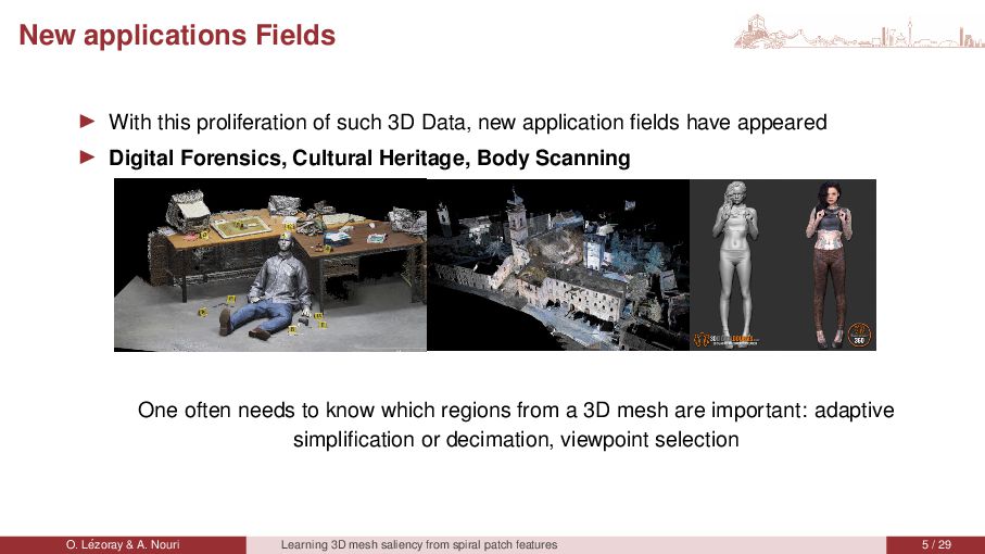
Data, new application fields have appeared ▶ Digital Forensics, Cultural Heritage, Body Scanning One often needs to know which regions from a 3D mesh are important: adaptive simplification or decimation, viewpoint selection O. L´ ezoray & A. Nouri Learning 3D mesh saliency from spiral patch features 5 / 29
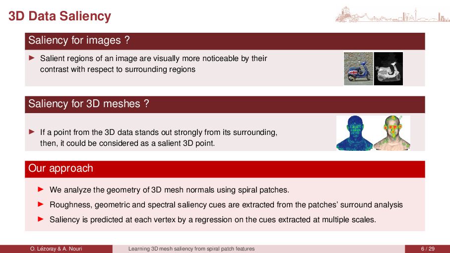
of an image are visually more noticeable by their contrast with respect to surrounding regions Saliency for 3D meshes ? ▶ If a point from the 3D data stands out strongly from its surrounding, then, it could be considered as a salient 3D point. Our approach ▶ We analyze the geometry of 3D mesh normals using spiral patches. ▶ Roughness, geometric and spectral saliency cues are extracted from the patches’ surround analysis ▶ Saliency is predicted at each vertex by a regression on the cues extracted at multiple scales. O. L´ ezoray & A. Nouri Learning 3D mesh saliency from spiral patch features 6 / 29
spectral saliencies 4. Saliency learning from multi-scale spiral cues O. L´ ezoray & A. Nouri Learning 3D mesh saliency from spiral patch features 7 / 29
spectral saliencies 4. Saliency learning from multi-scale spiral cues O. L´ ezoray & A. Nouri Learning 3D mesh saliency from spiral patch features 8 / 29
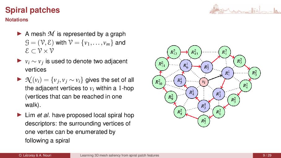
a graph G = (V,E) with V = {v1,...,vm } and E ⊂ V×V ▶ vi ∼ vj is used to denote two adjacent vertices ▶ N (vi ) = {vj,vj ∼ vi } gives the set of all the adjacent vertices to vi within a 1-hop (vertices that can be reached in one walk). ▶ Lim et al. have proposed local spiral hop descriptors: the surrounding vertices of one vertex can be enumerated by following a spiral O. L´ ezoray & A. Nouri Learning 3D mesh saliency from spiral patch features 9 / 29
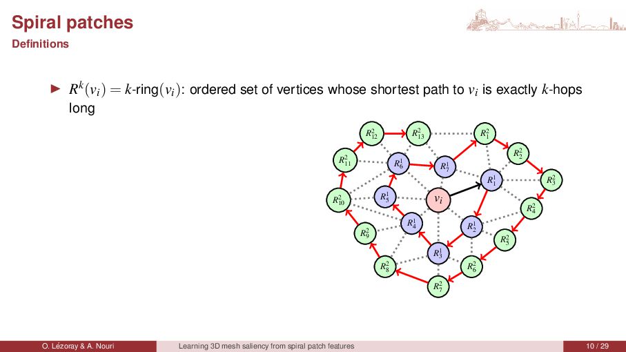
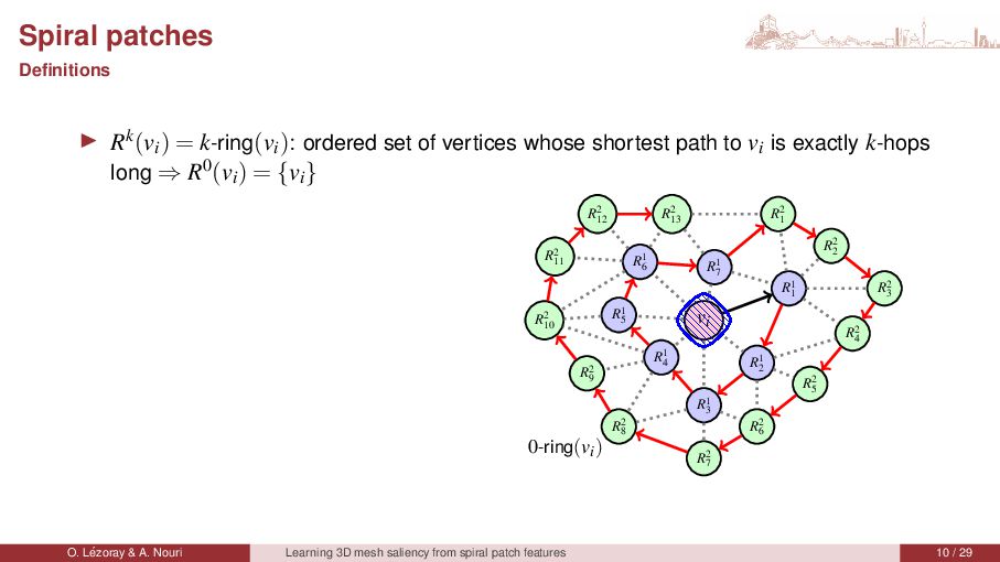
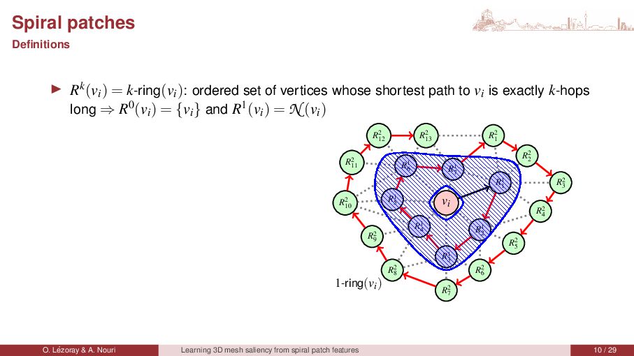
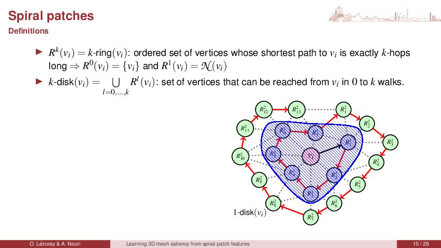
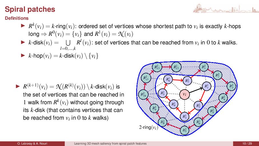
set of vertices whose shortest path to vi is exactly k-hops long ⇒ R0(vi ) = {vi } and R1(vi ) = N (vi ) ▶ k-disk(vi ) = l=0,...,k Rl(vi ): set of vertices that can be reached from vi in 0 to k walks. vi R1 7 R1 1 R1 2 R1 3 R1 4 R1 5 R1 6 R2 1 R2 2 R2 3 R2 4 R2 5 R2 6 R2 7 R2 8 R2 9 R2 10 R2 11 R2 12 R2 13 1-disk(vi) O. L´ ezoray & A. Nouri Learning 3D mesh saliency from spiral patch features 10 / 29
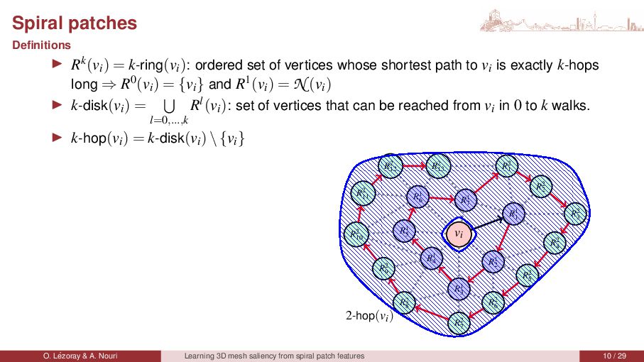
set of vertices whose shortest path to vi is exactly k-hops long ⇒ R0(vi ) = {vi } and R1(vi ) = N (vi ) ▶ k-disk(vi ) = l=0,...,k Rl(vi ): set of vertices that can be reached from vi in 0 to k walks. ▶ k-hop(vi ) = k-disk(vi )\{vi } vi R1 7 R1 1 R1 2 R1 3 R1 4 R1 5 R1 6 R2 1 R2 2 R2 3 R2 4 R2 5 R2 6 R2 7 R2 8 R2 9 R2 10 R2 11 R2 12 R2 13 2-hop(vi) O. L´ ezoray & A. Nouri Learning 3D mesh saliency from spiral patch features 10 / 29
set of vertices whose shortest path to vi is exactly k-hops long ⇒ R0(vi ) = {vi } and R1(vi ) = N (vi ) ▶ k-disk(vi ) = l=0,...,k Rl(vi ): set of vertices that can be reached from vi in 0 to k walks. ▶ k-hop(vi ) = k-disk(vi )\{vi } ▶ R(k+1)(vi ) = N (R(k)(vi ))\k-disk(vi ) is the set of vertices that can be reached in 1 walk from Rk(vi ) without going through its k-disk (that contains vertices that can be reached from vi in 0 to k walks) vi R1 7 R1 1 R1 2 R1 3 R1 4 R1 5 R1 6 R2 1 R2 2 R2 3 R2 4 R2 5 R2 6 R2 7 R2 8 R2 9 R2 10 R2 11 R2 12 R2 13 2-ring(vi) O. L´ ezoray & A. Nouri Learning 3D mesh saliency from spiral patch features 10 / 29
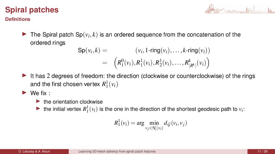
ordered sequence from the concatenation of the ordered rings Sp(vi,k) = (vi,1-ring(vi ),...,k-ring(vi )) = R0 1 (vi ),R1 1 (vi ),R1 2 (vi ),...,Rk |Rk| (vi ) ▶ It has 2 degrees of freedom: the direction (clockwise or counterclockwise) of the rings and the first chosen vertex R1 1 (vi ) ▶ We fix : ▶ the orientation clockwise ▶ the initial vertex R1 1 (vi ) is the one in the direction of the shortest geodesic path to vi: R1 1 (vi ) = arg min vj∈N (vi) dG(vi,vj ) O. L´ ezoray & A. Nouri Learning 3D mesh saliency from spiral patch features 11 / 29
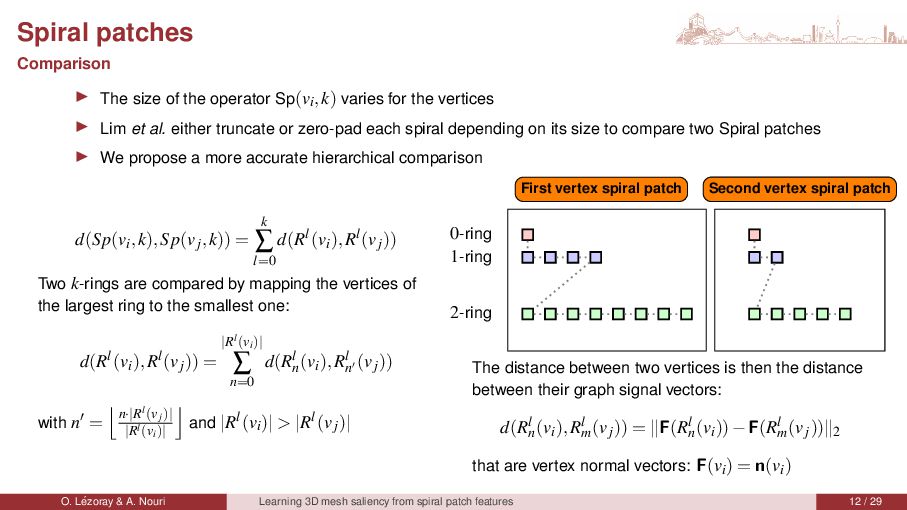
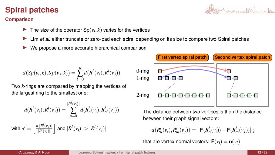
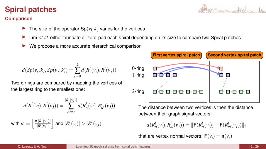
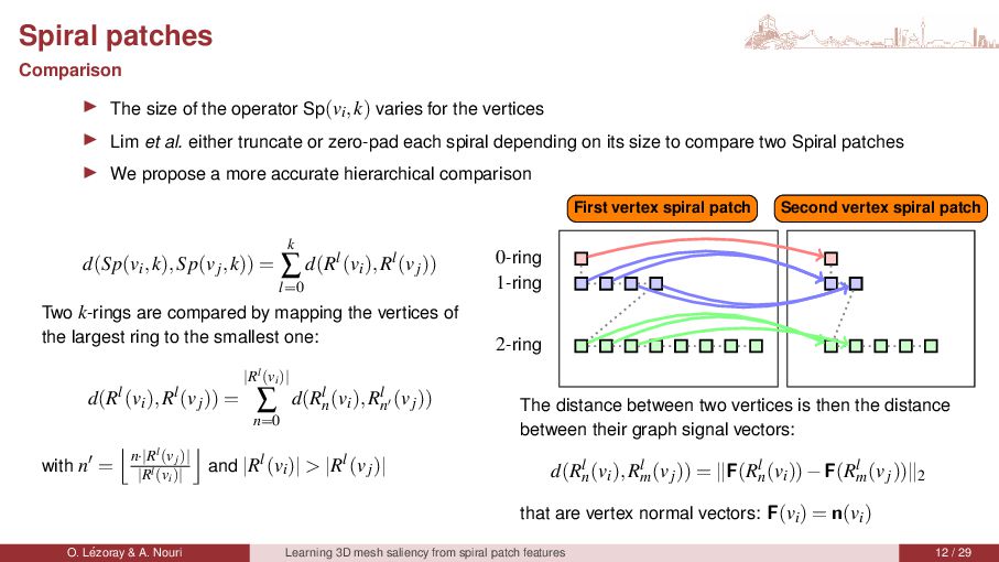
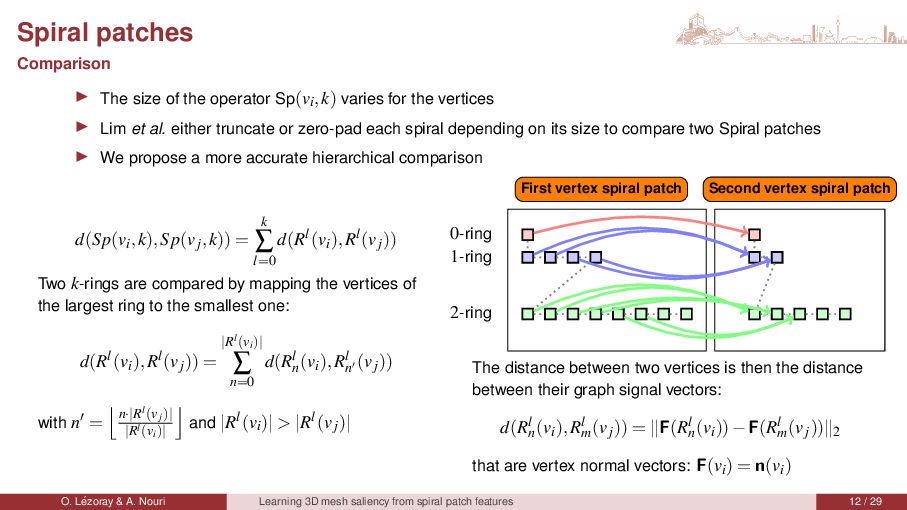
varies for the vertices ▶ Lim et al. either truncate or zero-pad each spiral depending on its size to compare two Spiral patches ▶ We propose a more accurate hierarchical comparison d(Sp(vi,k),Sp(vj,k)) = k ∑ l=0 d(Rl(vi),Rl(vj)) Two k-rings are compared by mapping the vertices of the largest ring to the smallest one: d(Rl(vi),Rl(vj)) = |Rl (vi )| ∑ n=0 d(Rl n (vi),Rl n′ (vj)) with n′ = n·|Rl (vj )| |Rl (vi )| and |Rl(vi)| > |Rl(vj)| First vertex spiral patch Second vertex spiral patch 0-ring 1-ring 2-ring The distance between two vertices is then the distance between their graph signal vectors: d(Rl n (vi),Rl m (vj)) = ∥F(Rl n (vi))−F(Rl m (vj))∥2 that are vertex normal vectors: F(vi) = n(vi) O. L´ ezoray & A. Nouri Learning 3D mesh saliency from spiral patch features 12 / 29
varies for the vertices ▶ Lim et al. either truncate or zero-pad each spiral depending on its size to compare two Spiral patches ▶ We propose a more accurate hierarchical comparison d(Sp(vi,k),Sp(vj,k)) = k ∑ l=0 d(Rl(vi),Rl(vj)) Two k-rings are compared by mapping the vertices of the largest ring to the smallest one: d(Rl(vi),Rl(vj)) = |Rl (vi )| ∑ n=0 d(Rl n (vi),Rl n′ (vj)) with n′ = n·|Rl (vj )| |Rl (vi )| and |Rl(vi)| > |Rl(vj)| First vertex spiral patch Second vertex spiral patch 0-ring 1-ring 2-ring The distance between two vertices is then the distance between their graph signal vectors: d(Rl n (vi),Rl m (vj)) = ∥F(Rl n (vi))−F(Rl m (vj))∥2 that are vertex normal vectors: F(vi) = n(vi) O. L´ ezoray & A. Nouri Learning 3D mesh saliency from spiral patch features 12 / 29
varies for the vertices ▶ Lim et al. either truncate or zero-pad each spiral depending on its size to compare two Spiral patches ▶ We propose a more accurate hierarchical comparison d(Sp(vi,k),Sp(vj,k)) = k ∑ l=0 d(Rl(vi),Rl(vj)) Two k-rings are compared by mapping the vertices of the largest ring to the smallest one: d(Rl(vi),Rl(vj)) = |Rl (vi )| ∑ n=0 d(Rl n (vi),Rl n′ (vj)) with n′ = n·|Rl (vj )| |Rl (vi )| and |Rl(vi)| > |Rl(vj)| First vertex spiral patch Second vertex spiral patch 0-ring 1-ring 2-ring The distance between two vertices is then the distance between their graph signal vectors: d(Rl n (vi),Rl m (vj)) = ∥F(Rl n (vi))−F(Rl m (vj))∥2 that are vertex normal vectors: F(vi) = n(vi) O. L´ ezoray & A. Nouri Learning 3D mesh saliency from spiral patch features 12 / 29
varies for the vertices ▶ Lim et al. either truncate or zero-pad each spiral depending on its size to compare two Spiral patches ▶ We propose a more accurate hierarchical comparison d(Sp(vi,k),Sp(vj,k)) = k ∑ l=0 d(Rl(vi),Rl(vj)) Two k-rings are compared by mapping the vertices of the largest ring to the smallest one: d(Rl(vi),Rl(vj)) = |Rl (vi )| ∑ n=0 d(Rl n (vi),Rl n′ (vj)) with n′ = n·|Rl (vj )| |Rl (vi )| and |Rl(vi)| > |Rl(vj)| First vertex spiral patch Second vertex spiral patch 0-ring 1-ring 2-ring The distance between two vertices is then the distance between their graph signal vectors: d(Rl n (vi),Rl m (vj)) = ∥F(Rl n (vi))−F(Rl m (vj))∥2 that are vertex normal vectors: F(vi) = n(vi) O. L´ ezoray & A. Nouri Learning 3D mesh saliency from spiral patch features 12 / 29
varies for the vertices ▶ Lim et al. either truncate or zero-pad each spiral depending on its size to compare two Spiral patches ▶ We propose a more accurate hierarchical comparison d(Sp(vi,k),Sp(vj,k)) = k ∑ l=0 d(Rl(vi),Rl(vj)) Two k-rings are compared by mapping the vertices of the largest ring to the smallest one: d(Rl(vi),Rl(vj)) = |Rl (vi )| ∑ n=0 d(Rl n (vi),Rl n′ (vj)) with n′ = n·|Rl (vj )| |Rl (vi )| and |Rl(vi)| > |Rl(vj)| First vertex spiral patch Second vertex spiral patch 0-ring 1-ring 2-ring The distance between two vertices is then the distance between their graph signal vectors: d(Rl n (vi),Rl m (vj)) = ∥F(Rl n (vi))−F(Rl m (vj))∥2 that are vertex normal vectors: F(vi) = n(vi) O. L´ ezoray & A. Nouri Learning 3D mesh saliency from spiral patch features 12 / 29
varies for the vertices ▶ Lim et al. either truncate or zero-pad each spiral depending on its size to compare two Spiral patches ▶ We propose a more accurate hierarchical comparison d(Sp(vi,k),Sp(vj,k)) = k ∑ l=0 d(Rl(vi),Rl(vj)) Two k-rings are compared by mapping the vertices of the largest ring to the smallest one: d(Rl(vi),Rl(vj)) = |Rl (vi )| ∑ n=0 d(Rl n (vi),Rl n′ (vj)) with n′ = n·|Rl (vj )| |Rl (vi )| and |Rl(vi)| > |Rl(vj)| First vertex spiral patch Second vertex spiral patch 0-ring 1-ring 2-ring The distance between two vertices is then the distance between their graph signal vectors: d(Rl n (vi),Rl m (vj)) = ∥F(Rl n (vi))−F(Rl m (vj))∥2 that are vertex normal vectors: F(vi) = n(vi) O. L´ ezoray & A. Nouri Learning 3D mesh saliency from spiral patch features 12 / 29
varies for the vertices ▶ Lim et al. either truncate or zero-pad each spiral depending on its size to compare two Spiral patches ▶ We propose a more accurate hierarchical comparison d(Sp(vi,k),Sp(vj,k)) = k ∑ l=0 d(Rl(vi),Rl(vj)) Two k-rings are compared by mapping the vertices of the largest ring to the smallest one: d(Rl(vi),Rl(vj)) = |Rl (vi )| ∑ n=0 d(Rl n (vi),Rl n′ (vj)) with n′ = n·|Rl (vj )| |Rl (vi )| and |Rl(vi)| > |Rl(vj)| First vertex spiral patch Second vertex spiral patch 0-ring 1-ring 2-ring The distance between two vertices is then the distance between their graph signal vectors: d(Rl n (vi),Rl m (vj)) = ∥F(Rl n (vi))−F(Rl m (vj))∥2 that are vertex normal vectors: F(vi) = n(vi) O. L´ ezoray & A. Nouri Learning 3D mesh saliency from spiral patch features 12 / 29
varies for the vertices ▶ Lim et al. either truncate or zero-pad each spiral depending on its size to compare two Spiral patches ▶ We propose a more accurate hierarchical comparison d(Sp(vi,k),Sp(vj,k)) = k ∑ l=0 d(Rl(vi),Rl(vj)) Two k-rings are compared by mapping the vertices of the largest ring to the smallest one: d(Rl(vi),Rl(vj)) = |Rl (vi )| ∑ n=0 d(Rl n (vi),Rl n′ (vj)) with n′ = n·|Rl (vj )| |Rl (vi )| and |Rl(vi)| > |Rl(vj)| First vertex spiral patch Second vertex spiral patch 0-ring 1-ring 2-ring The distance between two vertices is then the distance between their graph signal vectors: d(Rl n (vi),Rl m (vj)) = ∥F(Rl n (vi))−F(Rl m (vj))∥2 that are vertex normal vectors: F(vi) = n(vi) O. L´ ezoray & A. Nouri Learning 3D mesh saliency from spiral patch features 12 / 29
varies for the vertices ▶ Lim et al. either truncate or zero-pad each spiral depending on its size to compare two Spiral patches ▶ We propose a more accurate hierarchical comparison d(Sp(vi,k),Sp(vj,k)) = k ∑ l=0 d(Rl(vi),Rl(vj)) Two k-rings are compared by mapping the vertices of the largest ring to the smallest one: d(Rl(vi),Rl(vj)) = |Rl (vi )| ∑ n=0 d(Rl n (vi),Rl n′ (vj)) with n′ = n·|Rl (vj )| |Rl (vi )| and |Rl(vi)| > |Rl(vj)| First vertex spiral patch Second vertex spiral patch 0-ring 1-ring 2-ring The distance between two vertices is then the distance between their graph signal vectors: d(Rl n (vi),Rl m (vj)) = ∥F(Rl n (vi))−F(Rl m (vj))∥2 that are vertex normal vectors: F(vi) = n(vi) O. L´ ezoray & A. Nouri Learning 3D mesh saliency from spiral patch features 12 / 29
varies for the vertices ▶ Lim et al. either truncate or zero-pad each spiral depending on its size to compare two Spiral patches ▶ We propose a more accurate hierarchical comparison d(Sp(vi,k),Sp(vj,k)) = k ∑ l=0 d(Rl(vi),Rl(vj)) Two k-rings are compared by mapping the vertices of the largest ring to the smallest one: d(Rl(vi),Rl(vj)) = |Rl (vi )| ∑ n=0 d(Rl n (vi),Rl n′ (vj)) with n′ = n·|Rl (vj )| |Rl (vi )| and |Rl(vi)| > |Rl(vj)| First vertex spiral patch Second vertex spiral patch 0-ring 1-ring 2-ring The distance between two vertices is then the distance between their graph signal vectors: d(Rl n (vi),Rl m (vj)) = ∥F(Rl n (vi))−F(Rl m (vj))∥2 that are vertex normal vectors: F(vi) = n(vi) O. L´ ezoray & A. Nouri Learning 3D mesh saliency from spiral patch features 12 / 29
varies for the vertices ▶ Lim et al. either truncate or zero-pad each spiral depending on its size to compare two Spiral patches ▶ We propose a more accurate hierarchical comparison d(Sp(vi,k),Sp(vj,k)) = k ∑ l=0 d(Rl(vi),Rl(vj)) Two k-rings are compared by mapping the vertices of the largest ring to the smallest one: d(Rl(vi),Rl(vj)) = |Rl (vi )| ∑ n=0 d(Rl n (vi),Rl n′ (vj)) with n′ = n·|Rl (vj )| |Rl (vi )| and |Rl(vi)| > |Rl(vj)| First vertex spiral patch Second vertex spiral patch 0-ring 1-ring 2-ring The distance between two vertices is then the distance between their graph signal vectors: d(Rl n (vi),Rl m (vj)) = ∥F(Rl n (vi))−F(Rl m (vj))∥2 that are vertex normal vectors: F(vi) = n(vi) O. L´ ezoray & A. Nouri Learning 3D mesh saliency from spiral patch features 12 / 29
varies for the vertices ▶ Lim et al. either truncate or zero-pad each spiral depending on its size to compare two Spiral patches ▶ We propose a more accurate hierarchical comparison d(Sp(vi,k),Sp(vj,k)) = k ∑ l=0 d(Rl(vi),Rl(vj)) Two k-rings are compared by mapping the vertices of the largest ring to the smallest one: d(Rl(vi),Rl(vj)) = |Rl (vi )| ∑ n=0 d(Rl n (vi),Rl n′ (vj)) with n′ = n·|Rl (vj )| |Rl (vi )| and |Rl(vi)| > |Rl(vj)| First vertex spiral patch Second vertex spiral patch 0-ring 1-ring 2-ring The distance between two vertices is then the distance between their graph signal vectors: d(Rl n (vi),Rl m (vj)) = ∥F(Rl n (vi))−F(Rl m (vj))∥2 that are vertex normal vectors: F(vi) = n(vi) O. L´ ezoray & A. Nouri Learning 3D mesh saliency from spiral patch features 12 / 29
varies for the vertices ▶ Lim et al. either truncate or zero-pad each spiral depending on its size to compare two Spiral patches ▶ We propose a more accurate hierarchical comparison d(Sp(vi,k),Sp(vj,k)) = k ∑ l=0 d(Rl(vi),Rl(vj)) Two k-rings are compared by mapping the vertices of the largest ring to the smallest one: d(Rl(vi),Rl(vj)) = |Rl (vi )| ∑ n=0 d(Rl n (vi),Rl n′ (vj)) with n′ = n·|Rl (vj )| |Rl (vi )| and |Rl(vi)| > |Rl(vj)| First vertex spiral patch Second vertex spiral patch 0-ring 1-ring 2-ring The distance between two vertices is then the distance between their graph signal vectors: d(Rl n (vi),Rl m (vj)) = ∥F(Rl n (vi))−F(Rl m (vj))∥2 that are vertex normal vectors: F(vi) = n(vi) O. L´ ezoray & A. Nouri Learning 3D mesh saliency from spiral patch features 12 / 29
varies for the vertices ▶ Lim et al. either truncate or zero-pad each spiral depending on its size to compare two Spiral patches ▶ We propose a more accurate hierarchical comparison d(Sp(vi,k),Sp(vj,k)) = k ∑ l=0 d(Rl(vi),Rl(vj)) Two k-rings are compared by mapping the vertices of the largest ring to the smallest one: d(Rl(vi),Rl(vj)) = |Rl (vi )| ∑ n=0 d(Rl n (vi),Rl n′ (vj)) with n′ = n·|Rl (vj )| |Rl (vi )| and |Rl(vi)| > |Rl(vj)| First vertex spiral patch Second vertex spiral patch 0-ring 1-ring 2-ring The distance between two vertices is then the distance between their graph signal vectors: d(Rl n (vi),Rl m (vj)) = ∥F(Rl n (vi))−F(Rl m (vj))∥2 that are vertex normal vectors: F(vi) = n(vi) O. L´ ezoray & A. Nouri Learning 3D mesh saliency from spiral patch features 12 / 29
spectral saliencies 4. Saliency learning from multi-scale spiral cues O. L´ ezoray & A. Nouri Learning 3D mesh saliency from spiral patch features 14 / 29
spectral saliencies 4. Saliency learning from multi-scale spiral cues O. L´ ezoray & A. Nouri Learning 3D mesh saliency from spiral patch features 15 / 29
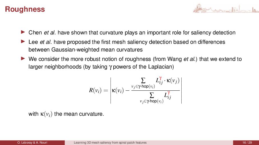
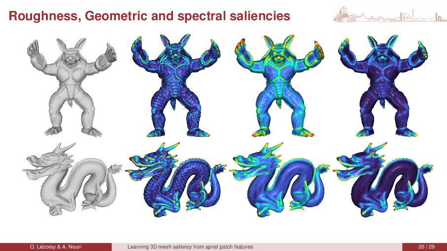
an important role for saliency detection ▶ Lee et al. have proposed the first mesh saliency detection based on differences between Gaussian-weighted mean curvatures ▶ We consider the more robust notion of roughness (from Wang et al.) that we extend to larger neighborhoods (by taking γ powers of the Laplacian) R(vi ) = κ(vi )− ∑ vj ∈γ-hop(vi ) Lγ i j ·κ(vj ) ∑ vj ∈γ-hop(vi ) Lγ i j with κ(vi ) the mean curvature. O. L´ ezoray & A. Nouri Learning 3D mesh saliency from spiral patch features 16 / 29
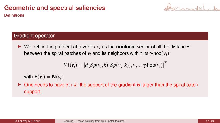
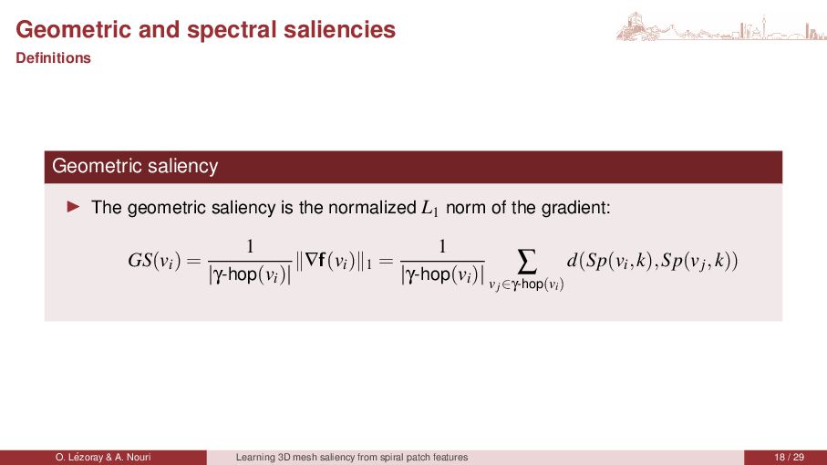
the gradient at a vertex vi as the nonlocal vector of all the distances between the spiral patches of vi and its neighbors within its γ-hop(vi ): ∇f(vi ) = [d(Sp(vi,k),Sp(vj,k)),vj ∈ γ-hop(vi )]T with F(vi ) = N(vi ) ▶ One needs to have γ > k: the support of the gradient is larger than the spiral patch support. O. L´ ezoray & A. Nouri Learning 3D mesh saliency from spiral patch features 17 / 29
saliency is the normalized L1 norm of the gradient: GS(vi ) = 1 |γ-hop(vi )| ∥∇f(vi )∥1 = 1 |γ-hop(vi )| ∑ vj ∈γ-hop(vi ) d(Sp(vi,k),Sp(vj,k)) O. L´ ezoray & A. Nouri Learning 3D mesh saliency from spiral patch features 18 / 29
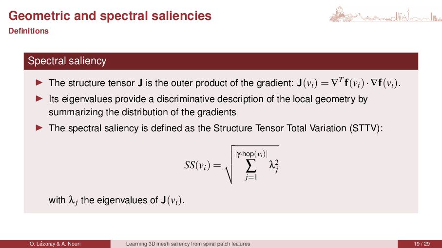
tensor J is the outer product of the gradient: J(vi ) = ∇T f(vi )·∇f(vi ). ▶ Its eigenvalues provide a discriminative description of the local geometry by summarizing the distribution of the gradients ▶ The spectral saliency is defined as the Structure Tensor Total Variation (STTV): SS(vi ) = |γ-hop(vi )| ∑ j=1 λ2 j with λj the eigenvalues of J(vi ). O. L´ ezoray & A. Nouri Learning 3D mesh saliency from spiral patch features 19 / 29
spectral saliencies 4. Saliency learning from multi-scale spiral cues O. L´ ezoray & A. Nouri Learning 3D mesh saliency from spiral patch features 21 / 29
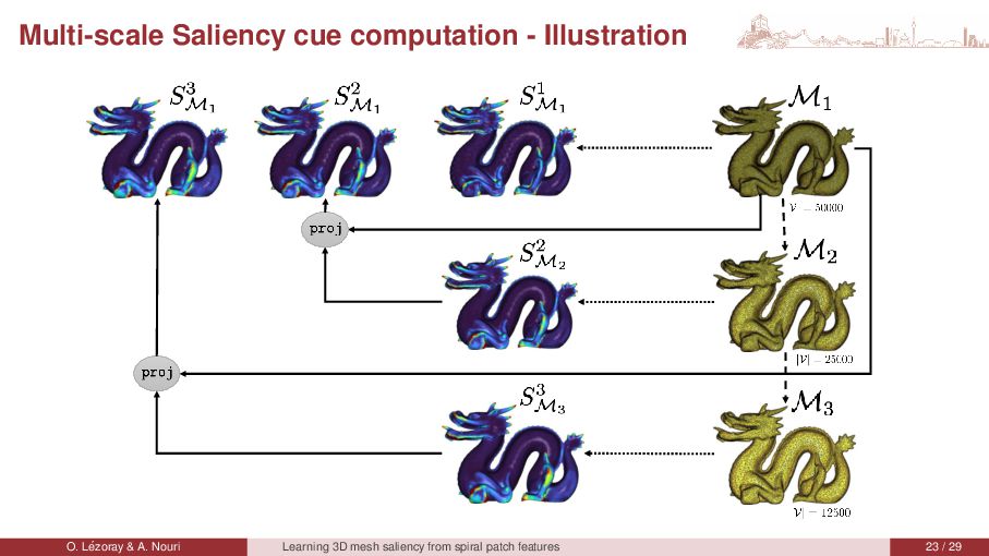
at three different resolutions obtained by mesh decimation with Qslim ▶ Given a mesh M1, we obtain meshes M2 and M3 with half and a quarter vertices ▶ We compute the saliency cues at each scale S1 M1 , S2 M2 , S3 M3 ▶ As the number of vertices decreases across scales, we cannot directly combine these computed multi-scale cues ▶ Given a saliency Sθ Mθ computed at scale θ, it is mapped back on the original mesh M1 by the projection Sθ M1 = proj(Sθ Mθ ,M1 ). ▶ This process yields three single-scale saliencies Sθ M1 for θ ∈ [1,3] O. L´ ezoray & A. Nouri Learning 3D mesh saliency from spiral patch features 22 / 29
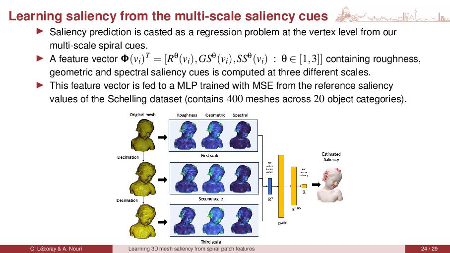
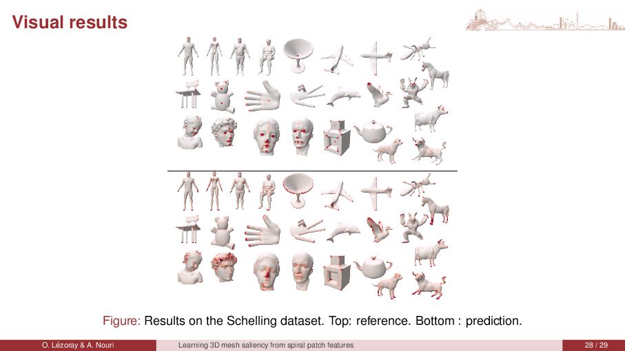
is casted as a regression problem at the vertex level from our multi-scale spiral cues. ▶ A feature vector Φ(vi )T = [Rθ(vi ),GSθ(vi ),SSθ(vi ) : θ ∈ [1,3]] containing roughness, geometric and spectral saliency cues is computed at three different scales. ▶ This feature vector is fed to a MLP trained with MSE from the reference saliency values of the Schelling dataset (contains 400 meshes across 20 object categories). O. L´ ezoray & A. Nouri Learning 3D mesh saliency from spiral patch features 24 / 29
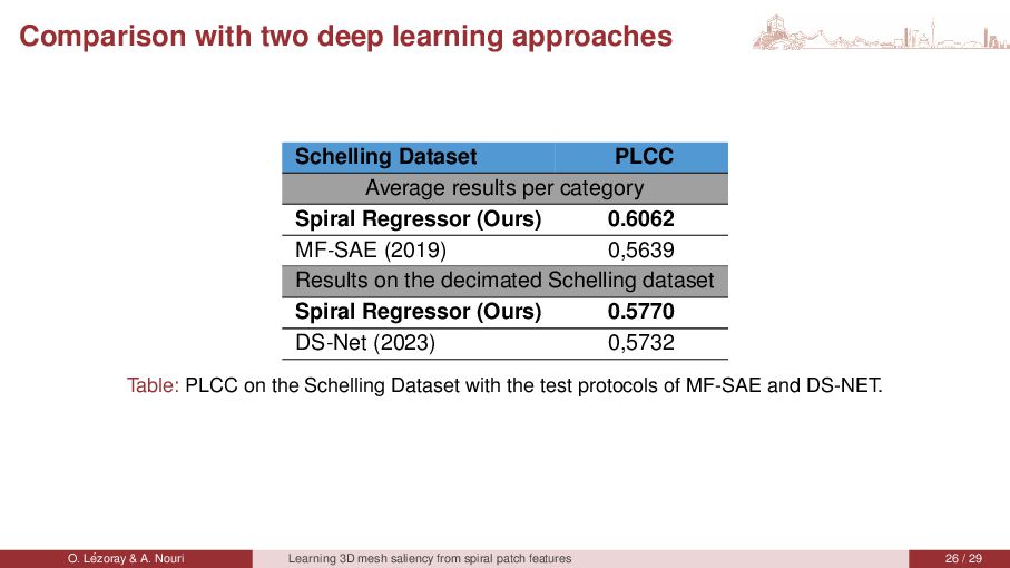
results per category Spiral Regressor (Ours) 0.6062 MF-SAE (2019) 0,5639 Results on the decimated Schelling dataset Spiral Regressor (Ours) 0.5770 DS-Net (2023) 0,5732 Table: PLCC on the Schelling Dataset with the test protocols of MF-SAE and DS-NET. O. L´ ezoray & A. Nouri Learning 3D mesh saliency from spiral patch features 26 / 29
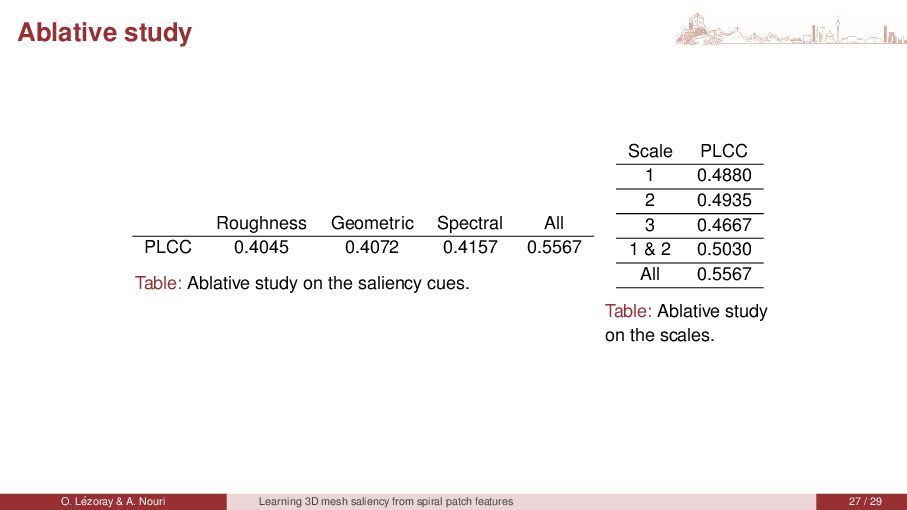
0.5567 Table: Ablative study on the saliency cues. Scale PLCC 1 0.4880 2 0.4935 3 0.4667 1 & 2 0.5030 All 0.5567 Table: Ablative study on the scales. O. L´ ezoray & A. Nouri Learning 3D mesh saliency from spiral patch features 27 / 29