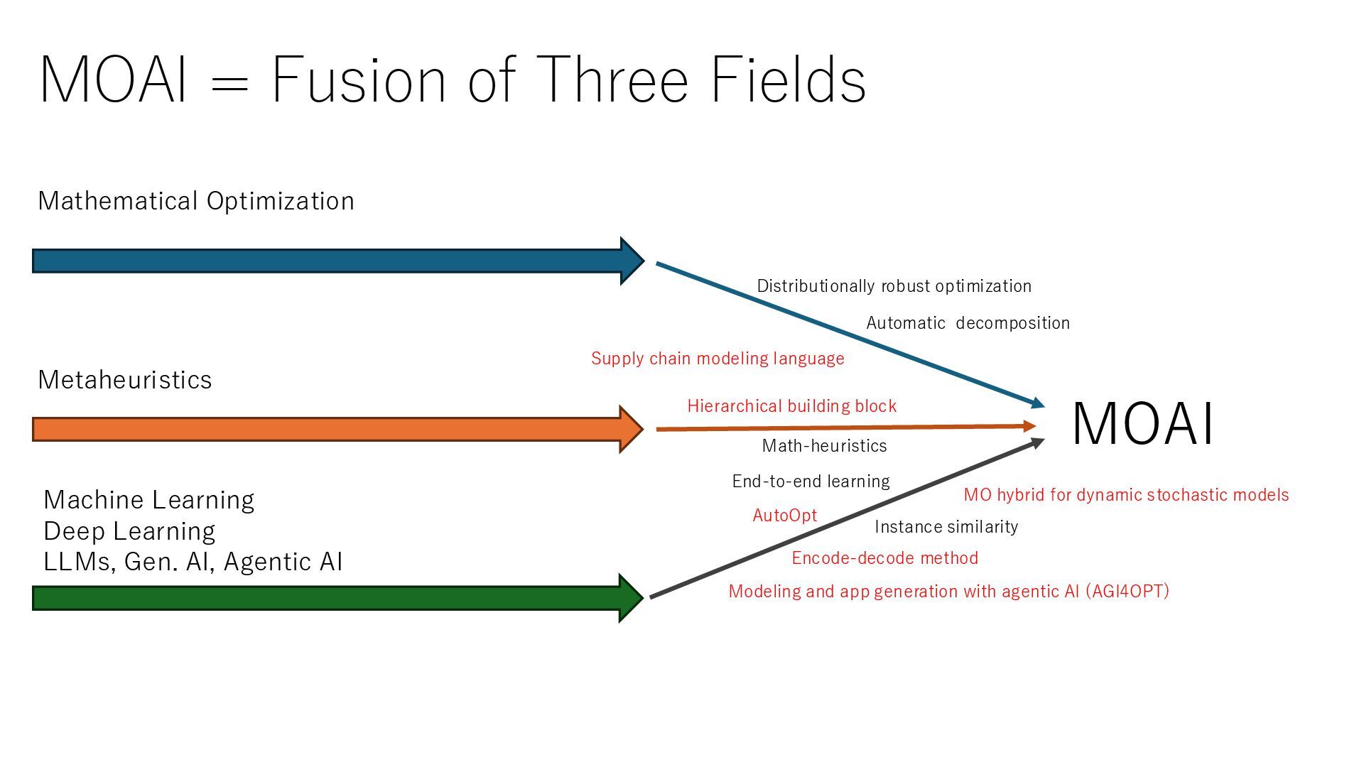
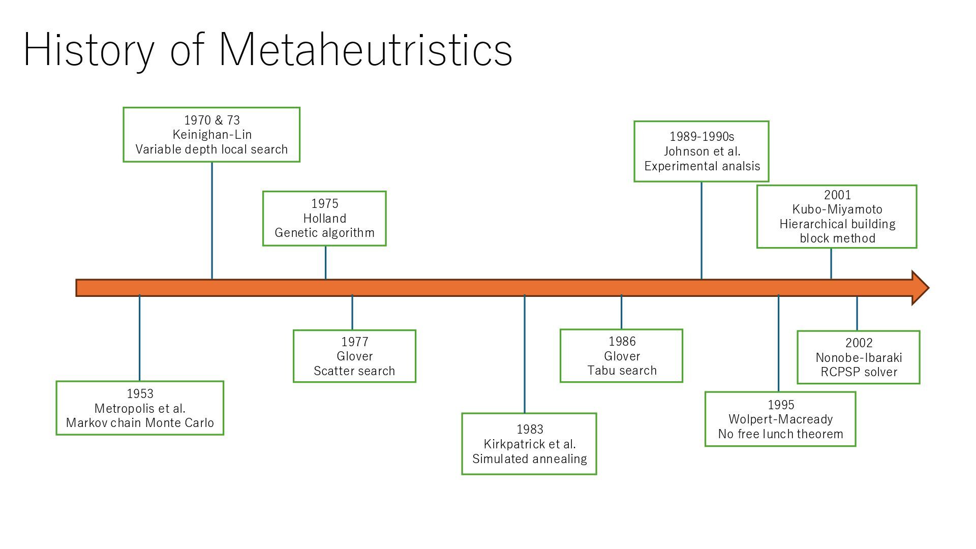
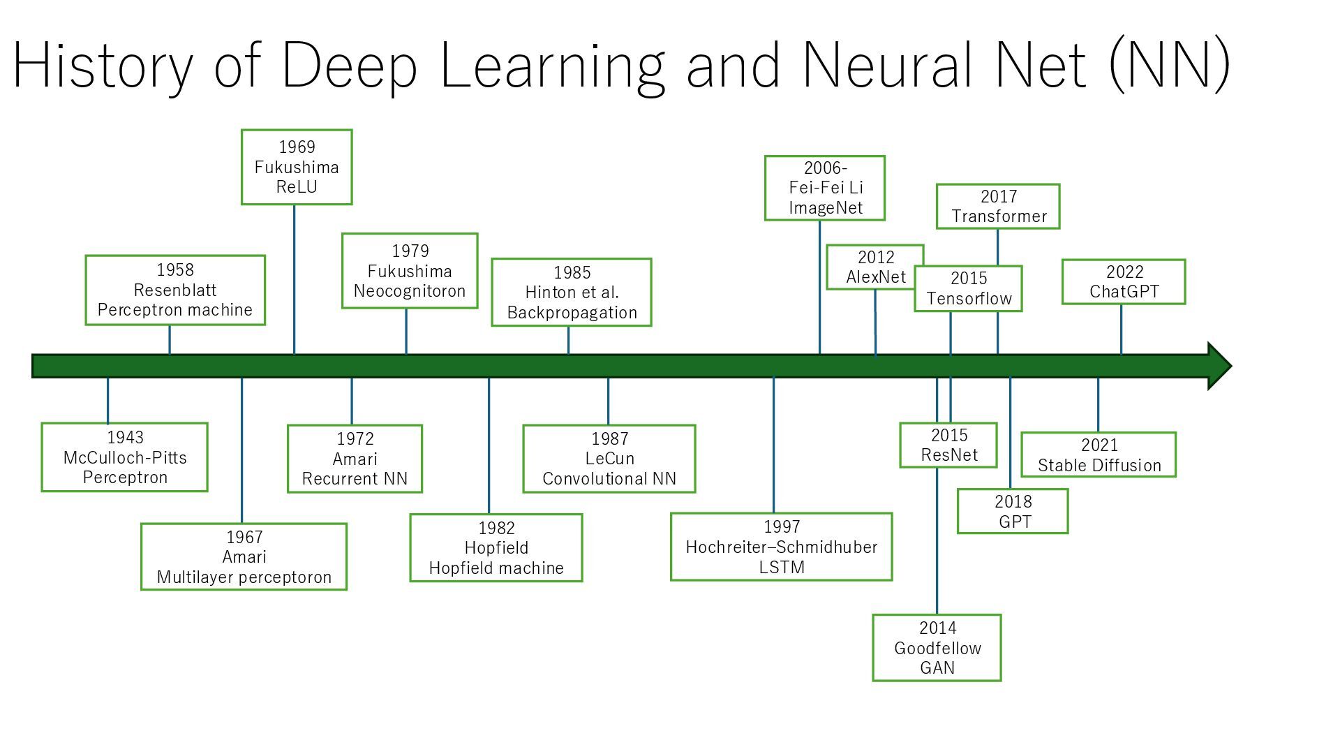
Learning Deep Learning LLMs, Gen. AI, Agentic AI MOAI Hierarchical building block AutoOpt Math-heuristics Distributionally robust optimization Encode-decode method MO hybrid for dynamic stochastic models End-to-end learning Supply chain modeling language Modeling and app generation with agentic AI (AGI4OPT) Automatic decomposition Instance similarity
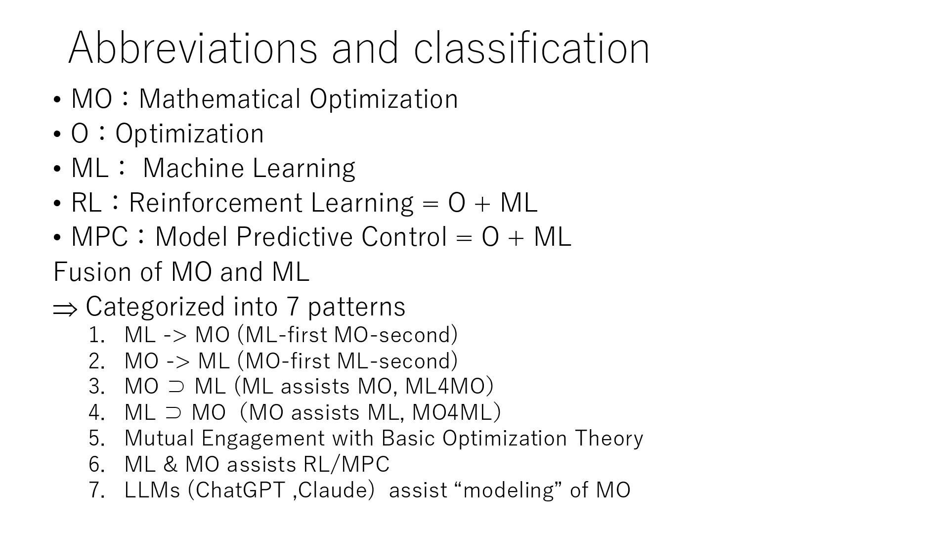
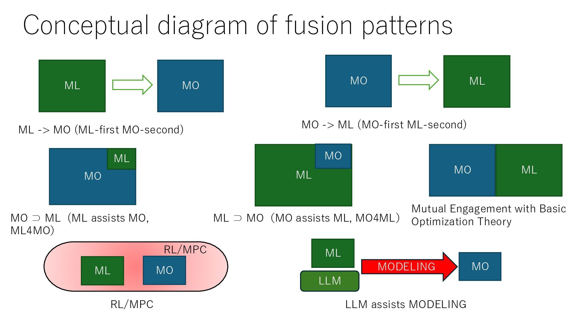
Machine Learning • RL:Reinforcement Learning = O + ML • MPC:Model Predictive Control = O + ML Fusion of MO and ML Categorized into 7 patterns 1. ML -> MO (ML-first MO-second) 2. MO -> ML (MO-first ML-second) 3. MO ⊃ ML (ML assists MO, ML4MO) 4. ML ⊃ MO(MO assists ML, MO4ML) 5. Mutual Engagement with Basic Optimization Theory 6. ML & MO assists RL/MPC 7. LLMs (ChatGPT ,Claude) assist “modeling” of MO
(ML-first MO-second) MO -> ML (MO-first ML-second) ML MO MO ⊃ ML (ML assists MO, ML4MO) ML ⊃ MO(MO assists ML, MO4ML) Mutual Engagement with Basic Optimization Theory RL/MPC MO ML MO ML ML MO ML MO RL/MPC LLM assists MODELING ML MO MODELING LLM
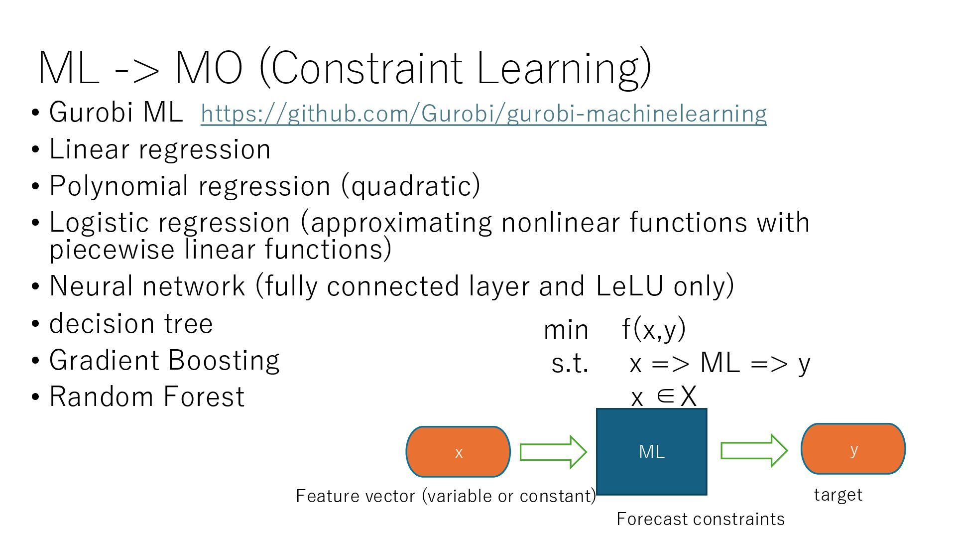
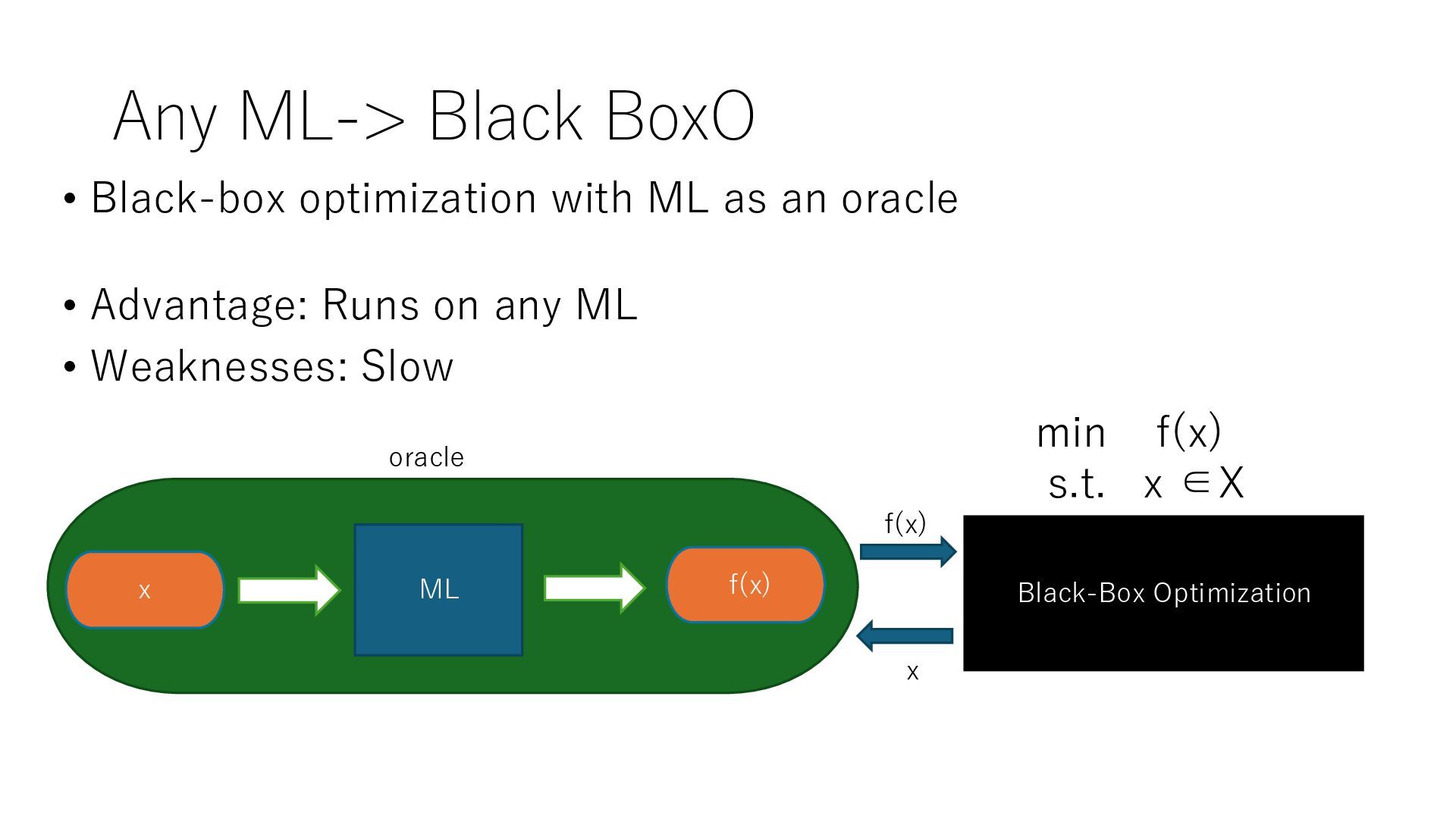
ML The most classic and natural (predict and then optimize) approach 1. Predict with ML and function approximation = > Solve the approximate constraint or objective function with MO ✓ Embedding ML prediction models as mathematical formulas in MO (Gurobi 10.0+) ✓ Optimize ML as a black box ✓ Approximate an ML prediction model as an MO-solvable function with realistic assumptions 2. Preprocessing with ML (e.g., clustering) → MO ML MO データ Solution
Linear regression • Polynomial regression (quadratic) • Logistic regression (approximating nonlinear functions with piecewise linear functions) • Neural network (fully connected layer and LeLU only) • decision tree • Gradient Boosting • Random Forest ML y x Feature vector (variable or constant) Forecast constraints target min f(x,y) s.t. x => ML => y x ∈X
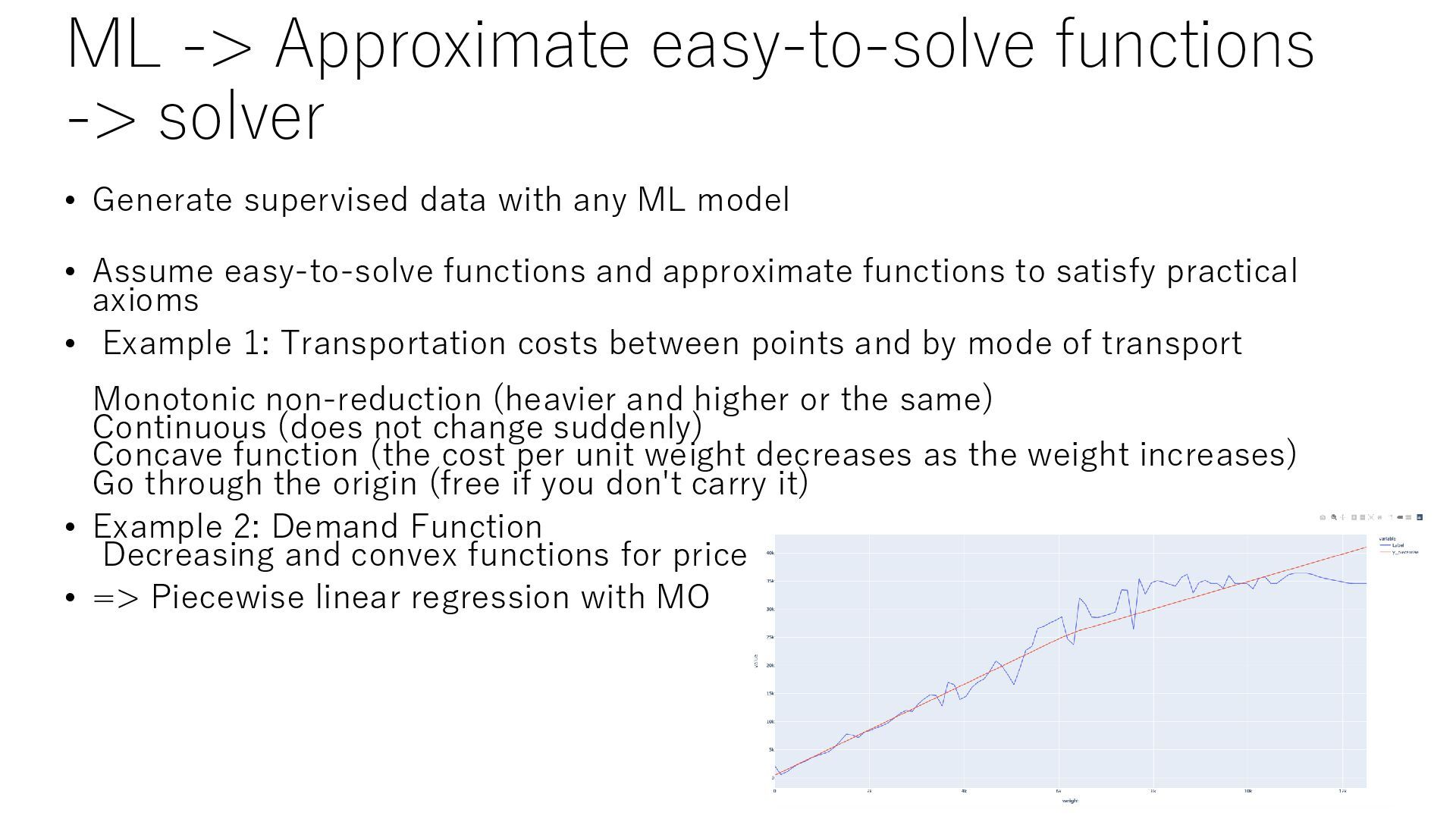
data with any ML model • Assume easy-to-solve functions and approximate functions to satisfy practical axioms • Example 1: Transportation costs between points and by mode of transport Monotonic non-reduction (heavier and higher or the same) Continuous (does not change suddenly) Concave function (the cost per unit weight decreases as the weight increases) Go through the origin (free if you don't carry it) • Example 2: Demand Function Decreasing and convex functions for price • => Piecewise linear regression with MO
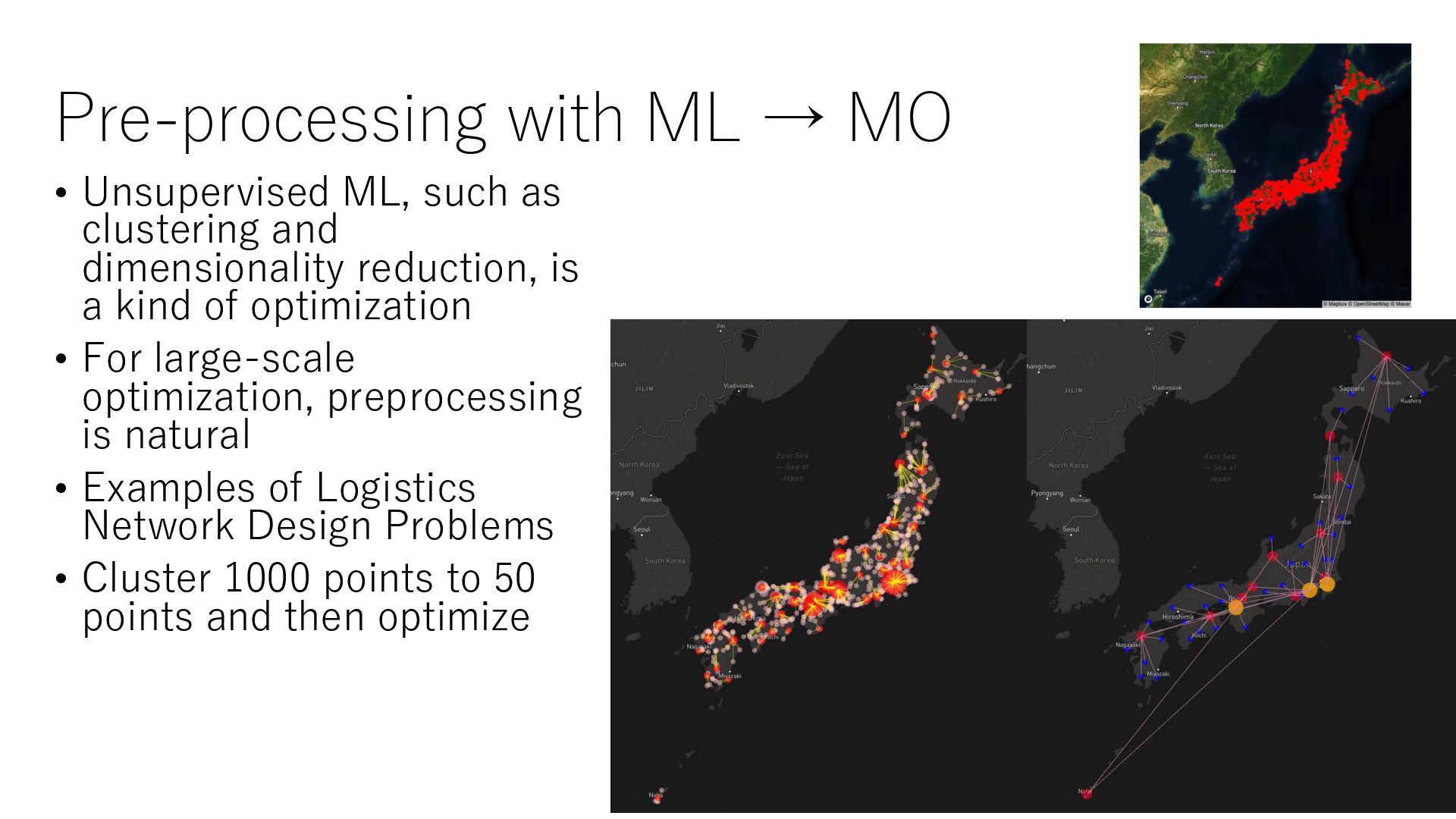
clustering and dimensionality reduction, is a kind of optimization • For large-scale optimization, preprocessing is natural • Examples of Logistics Network Design Problems • Cluster 1000 points to 50 points and then optimize
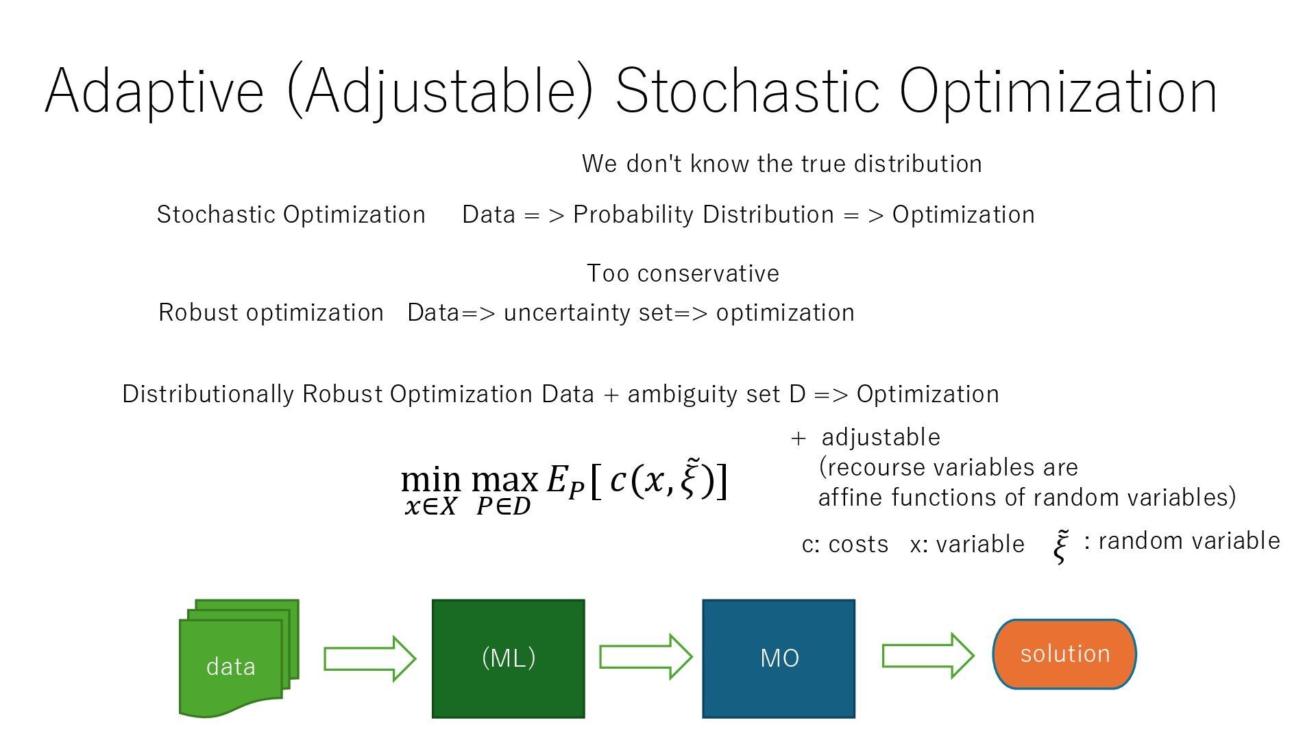
> Probability Distribution = > Optimization Robust optimization Data=> uncertainty set=> optimization Distributionally Robust Optimization Data + ambiguity set D => Optimization min 𝑥∈𝑋 max 𝑃∈𝐷 𝐸𝑃 [ 𝑐(𝑥, ሚ 𝜉)] c: costs x: variable (ML) MO data solution : random variable Too conservative We don't know the true distribution + adjustable (recourse variables are affine functions of random variables)
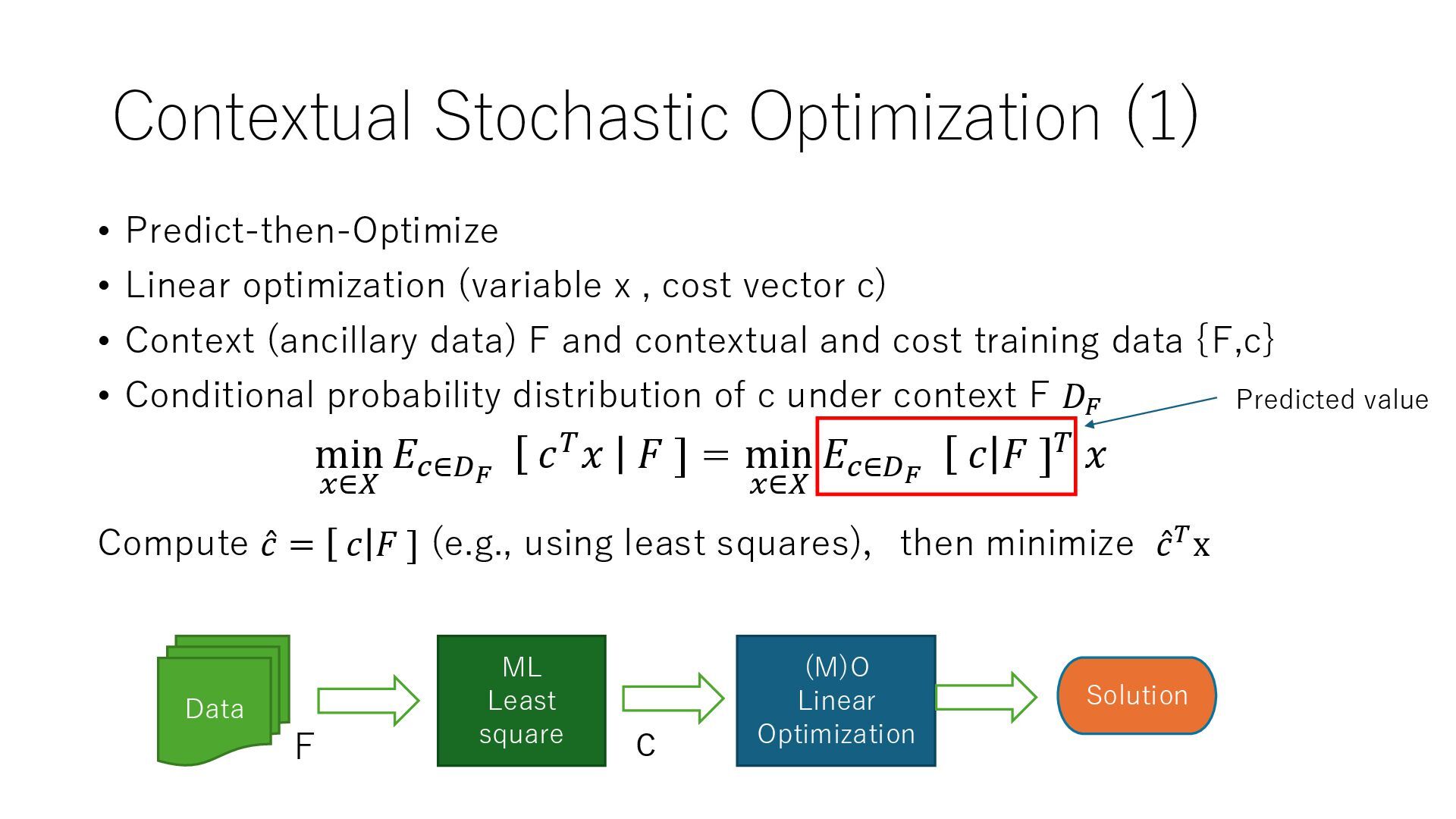
x , cost vector c) • Context (ancillary data) F and contextual and cost training data {F,c} • Conditional probability distribution of c under context F 𝐷𝐹 Compute Ƹ 𝑐 = 𝑐 𝐹 ] (e.g., using least squares),then minimize Ƹ 𝑐𝑇x min 𝑥∈𝑋 𝐸𝑐∈𝐷𝐹 𝑐𝑇𝑥 𝐹 ] = min 𝑥∈𝑋 𝐸𝑐∈𝐷𝐹 𝑐 𝐹 ]𝑇 𝑥 Predicted value ML Least square (M)O Linear Optimization Data Solution F c
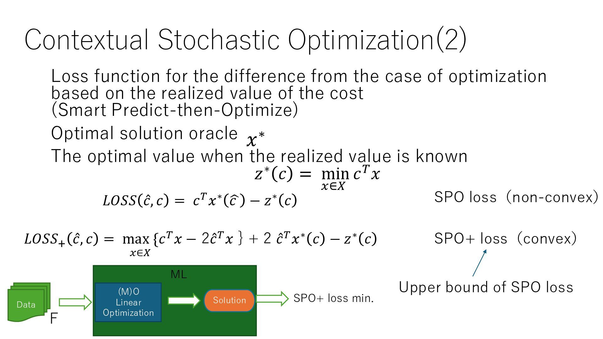
case of optimization based on the realized value of the cost (Smart Predict-then-Optimize) Optimal solution oracle The optimal value when the realized value is known 𝑧∗ 𝑐 = min 𝑥∈𝑋 𝑐𝑇𝑥 𝐿𝑂𝑆𝑆+ Ƹ 𝑐, 𝑐 = max { 𝑥∈𝑋 𝑐𝑇𝑥 − 2 Ƹ 𝑐𝑇𝑥 } + 2 Ƹ 𝑐𝑇𝑥∗ 𝑐 − 𝑧∗ 𝑐 𝐿𝑂𝑆𝑆 Ƹ 𝑐, 𝑐 = 𝑐𝑇𝑥∗ ෝ 𝑐 − 𝑧∗ 𝑐 SPO loss(non-convex) SPO+ loss(convex) 𝑥∗ Upper bound of SPO loss (M)O Linear Optimization Data Solution ML SPO+ loss min. F
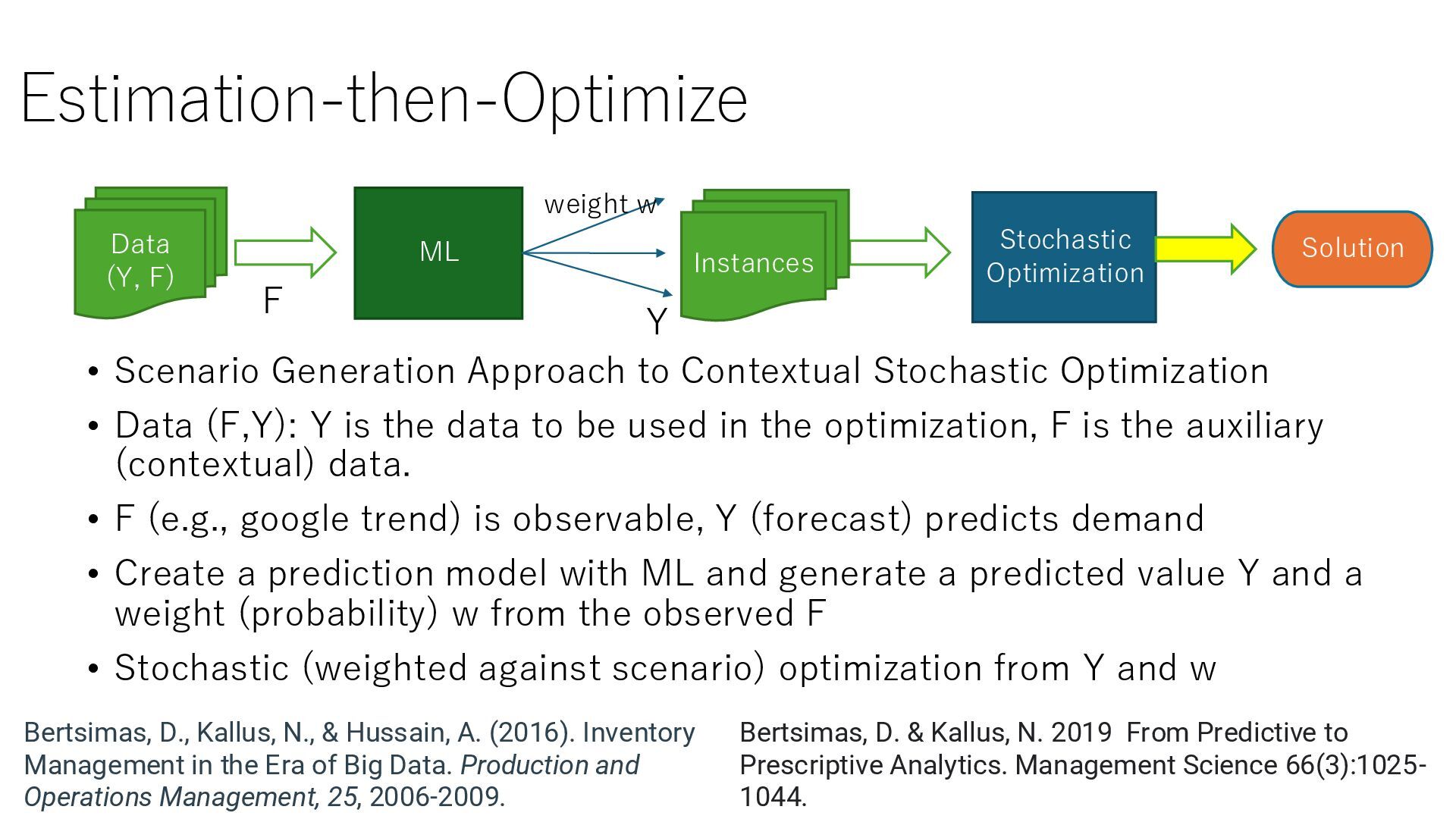
Data (F,Y): Y is the data to be used in the optimization, F is the auxiliary (contextual) data. • F (e.g., google trend) is observable, Y (forecast) predicts demand • Create a prediction model with ML and generate a predicted value Y and a weight (probability) w from the observed F • Stochastic (weighted against scenario) optimization from Y and w Bertsimas, D. & Kallus, N. 2019 From Predictive to Prescriptive Analytics. Management Science 66(3):1025- 1044. ML Stochastic Optimization Data (Y, F) Solution Instances weight w Bertsimas, D., Kallus, N., & Hussain, A. (2016). Inventory Management in the Era of Big Data. Production and Operations Management, 25, 2006-2009. F Y
models distributed robust optimization and contextual stochastic optimization https://xiongpengnus.github.io/rsome/ • Convert a min max type robust optimization model containing an uncertainty set or an ambiguity set into a deterministic optimization model and solve it.
model into MO increases the amount of computation. • Combining a large-scale ML model with a large-scale MO model is problem-dependent • Application examples are mainly simple ones such as inventory optimization
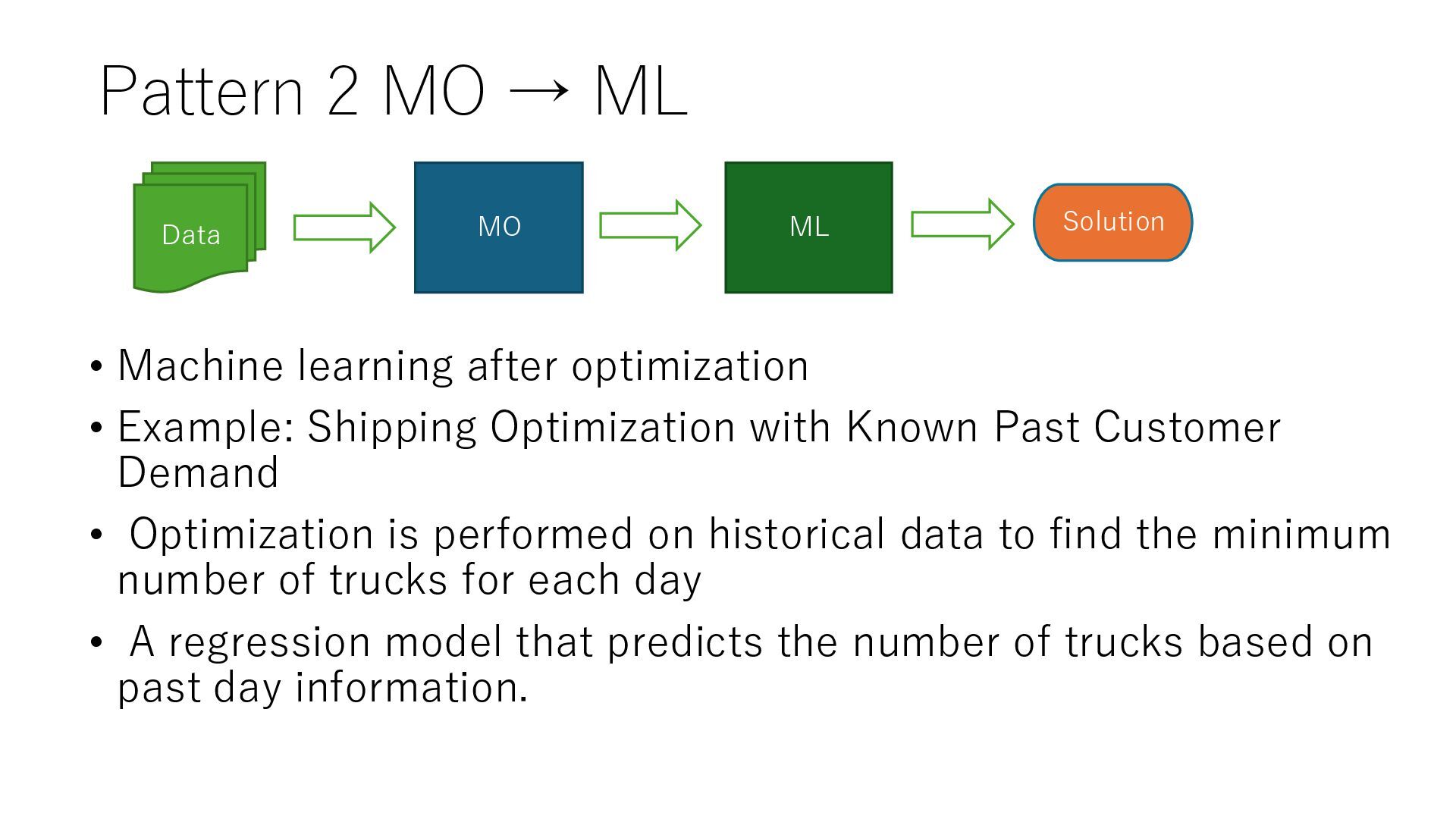
• Example: Shipping Optimization with Known Past Customer Demand • Optimization is performed on historical data to find the minimum number of trucks for each day • A regression model that predicts the number of trucks based on past day information. ML MO Data Solution
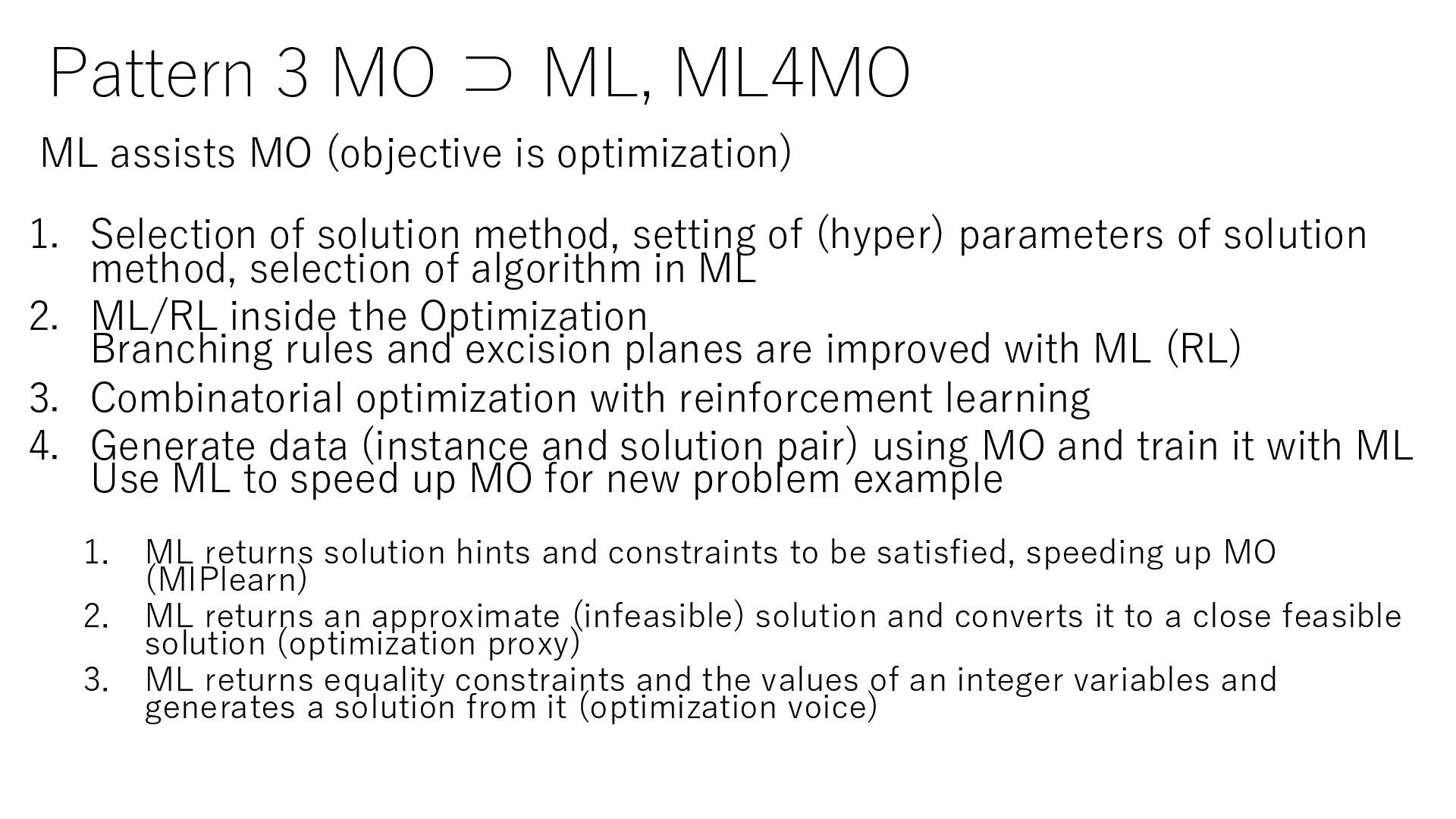
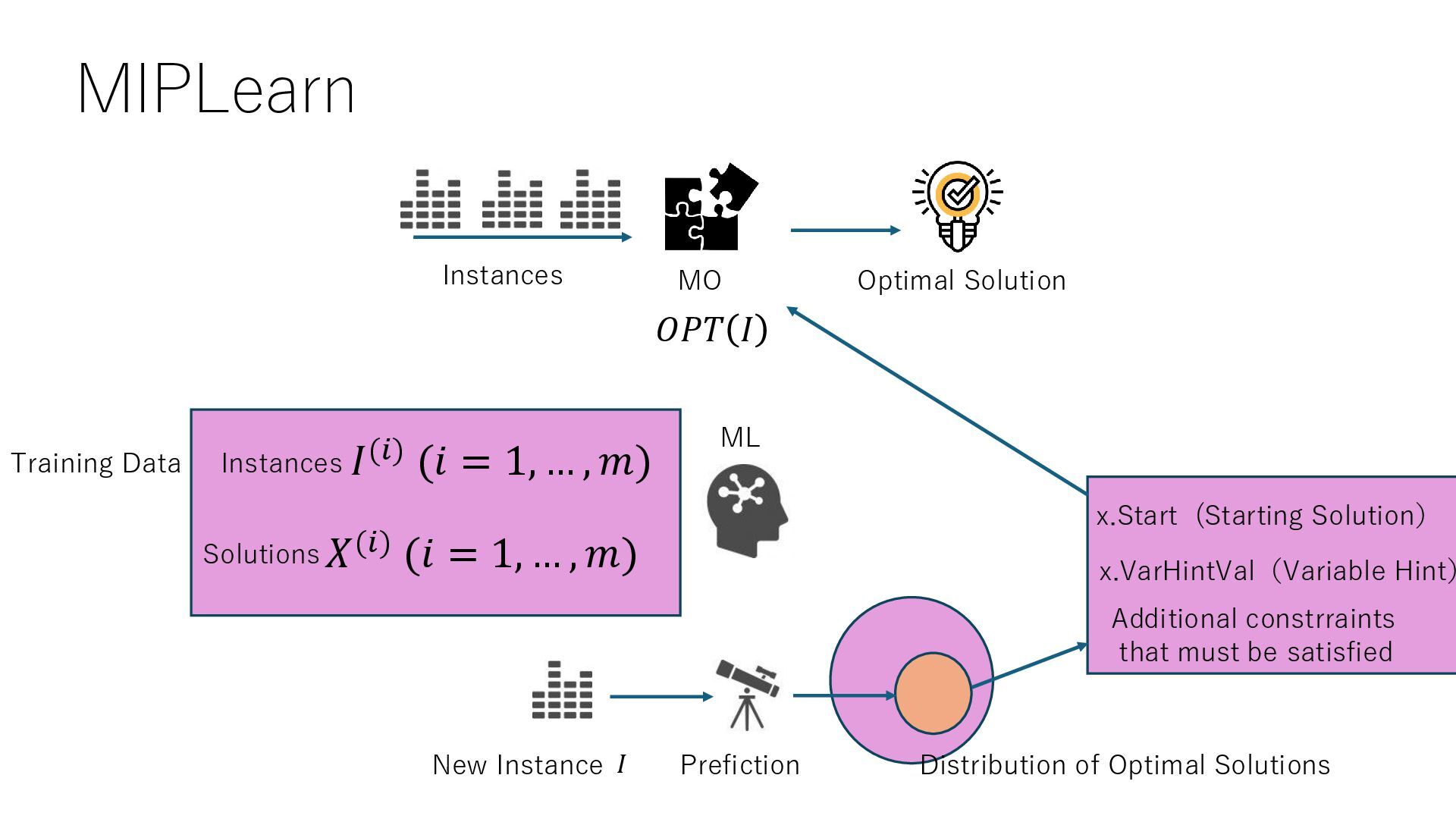
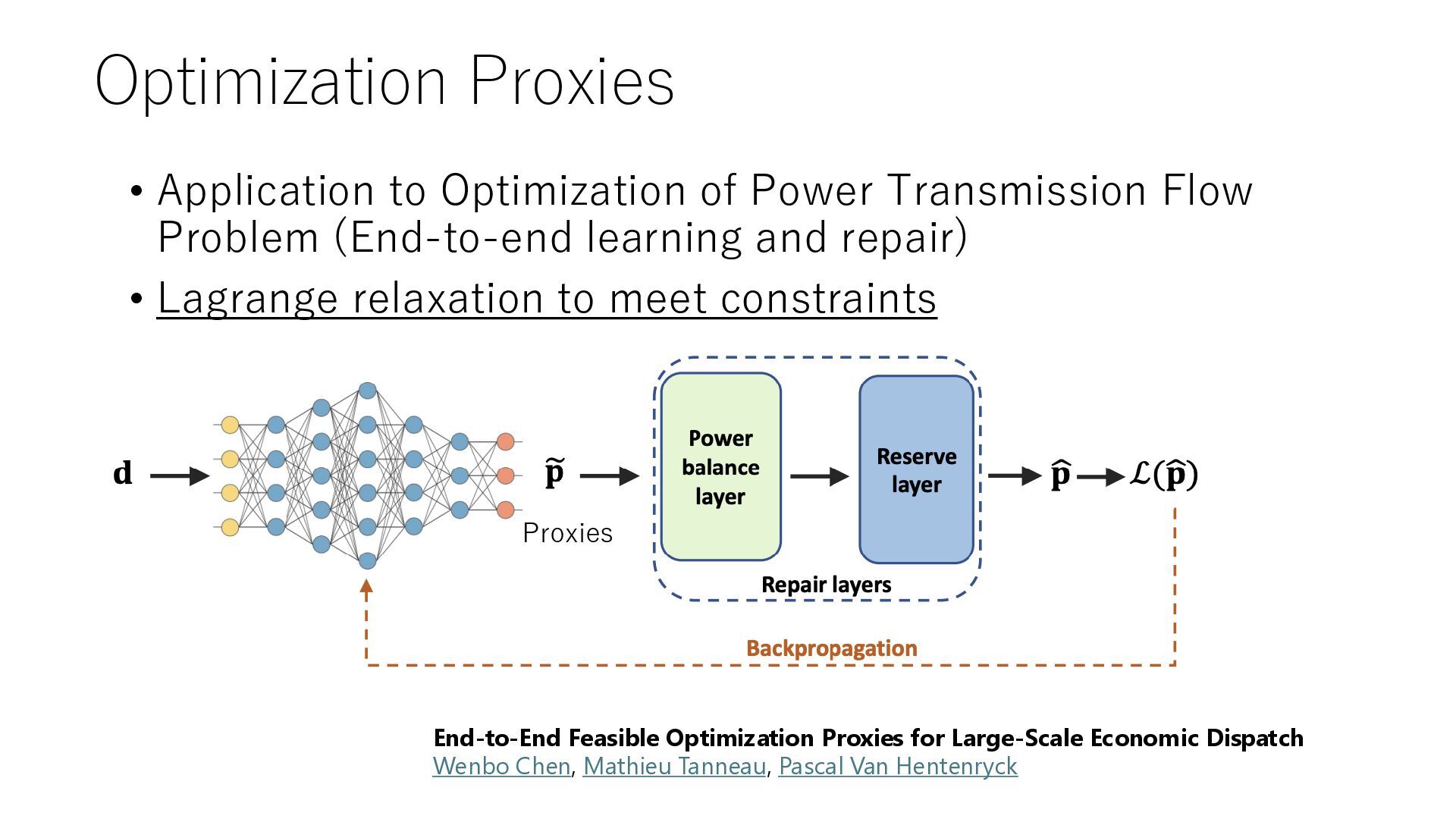
is optimization) 1. Selection of solution method, setting of (hyper) parameters of solution method, selection of algorithm in ML 2. ML/RL inside the Optimization Branching rules and excision planes are improved with ML (RL) 3. Combinatorial optimization with reinforcement learning 4. Generate data (instance and solution pair) using MO and train it with ML Use ML to speed up MO for new problem example 1. ML returns solution hints and constraints to be satisfied, speeding up MO (MIPlearn) 2. ML returns an approximate (infeasible) solution and converts it to a close feasible solution (optimization proxy) 3. ML returns equality constraints and the values of an integer variables and generates a solution from it (optimization voice)
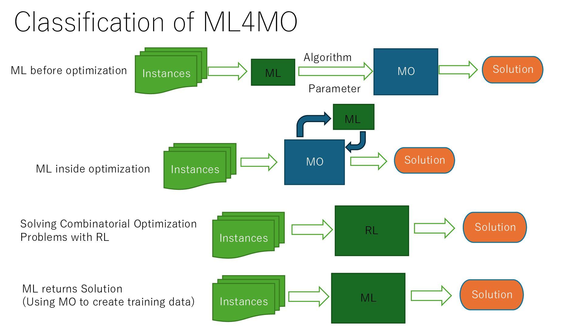
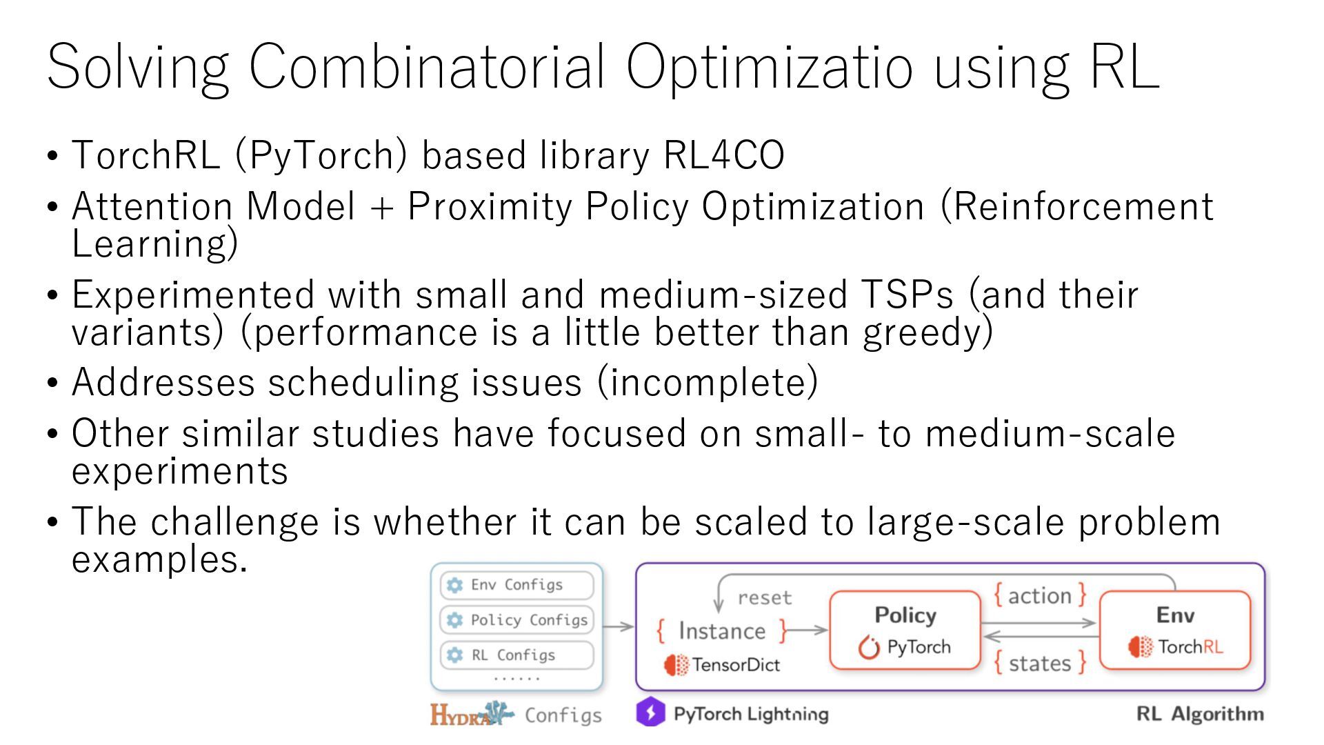
to create training data) MO Instances Solution ML Parameter Algorithm ML before optimization Instances Instances Instances MO Solution ML ML inside optimization Solution RL Solving Combinatorial Optimization Problems with RL
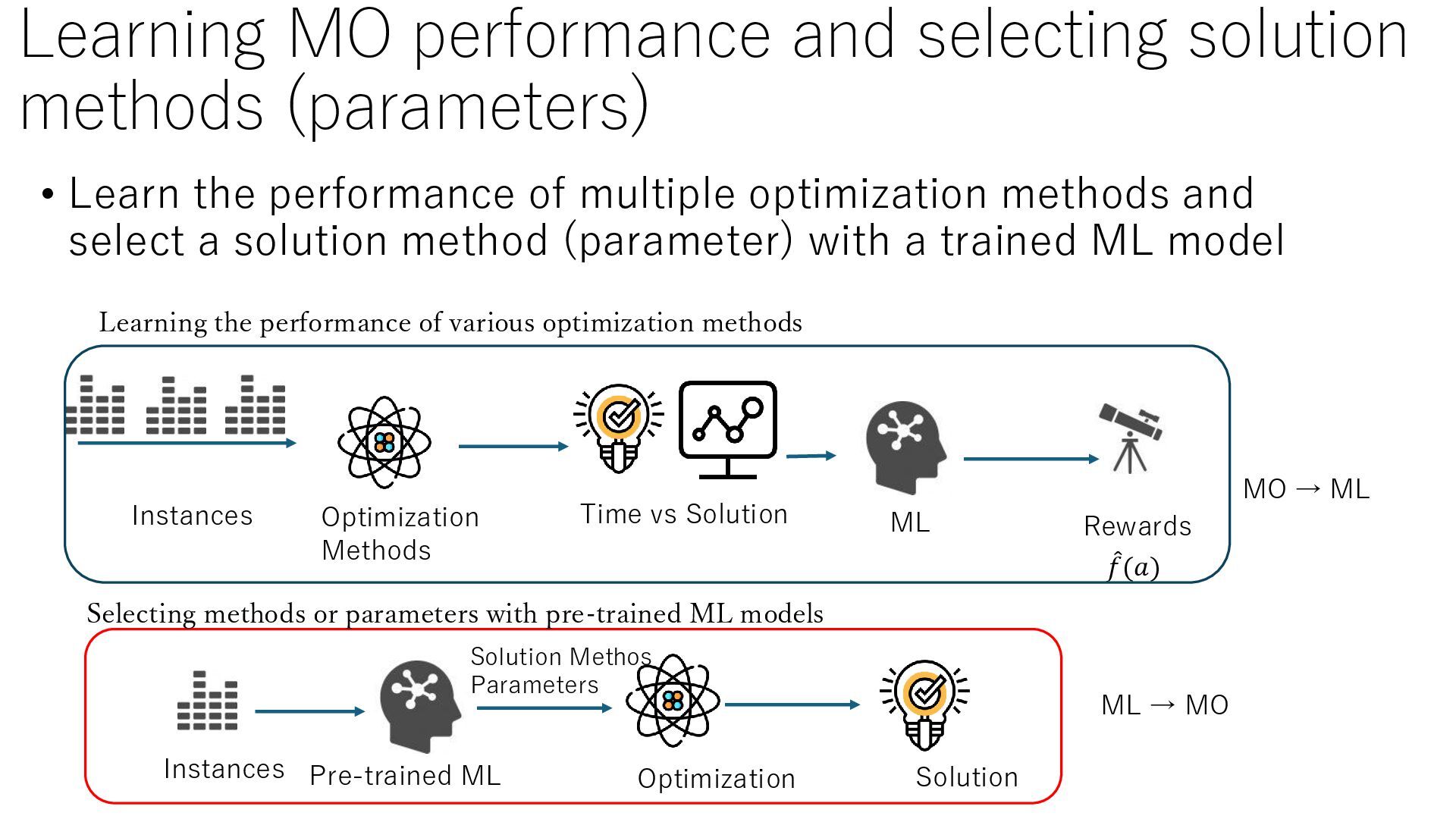
the performance of multiple optimization methods and select a solution method (parameter) with a trained ML model Instances ML Optimization Methods Time vs Solution Rewards Pre-trained ML መ 𝑓(𝑎) Learning the performance of various optimization methods Instances Optimization ML → MO MO → ML Solution Methos Parameters Solution Selecting methods or parameters with pre-trained ML models
RL4CO • Attention Model + Proximity Policy Optimization (Reinforcement Learning) • Experimented with small and medium-sized TSPs (and their variants) (performance is a little better than greedy) • Addresses scheduling issues (incomplete) • Other similar studies have focused on small- to medium-scale experiments • The challenge is whether it can be scaled to large-scale problem examples.
, 𝑚) 𝑂𝑃𝑇 𝐼 Optimal Solution 𝑋(𝑖) (𝑖 = 1, … , 𝑚) Instances Solutions Training Data New Instance Distribution of Optimal Solutions 𝐼 x.Start (Starting Solution) x.VarHintVal(Variable Hint) Additional constrraints that must be satisfied
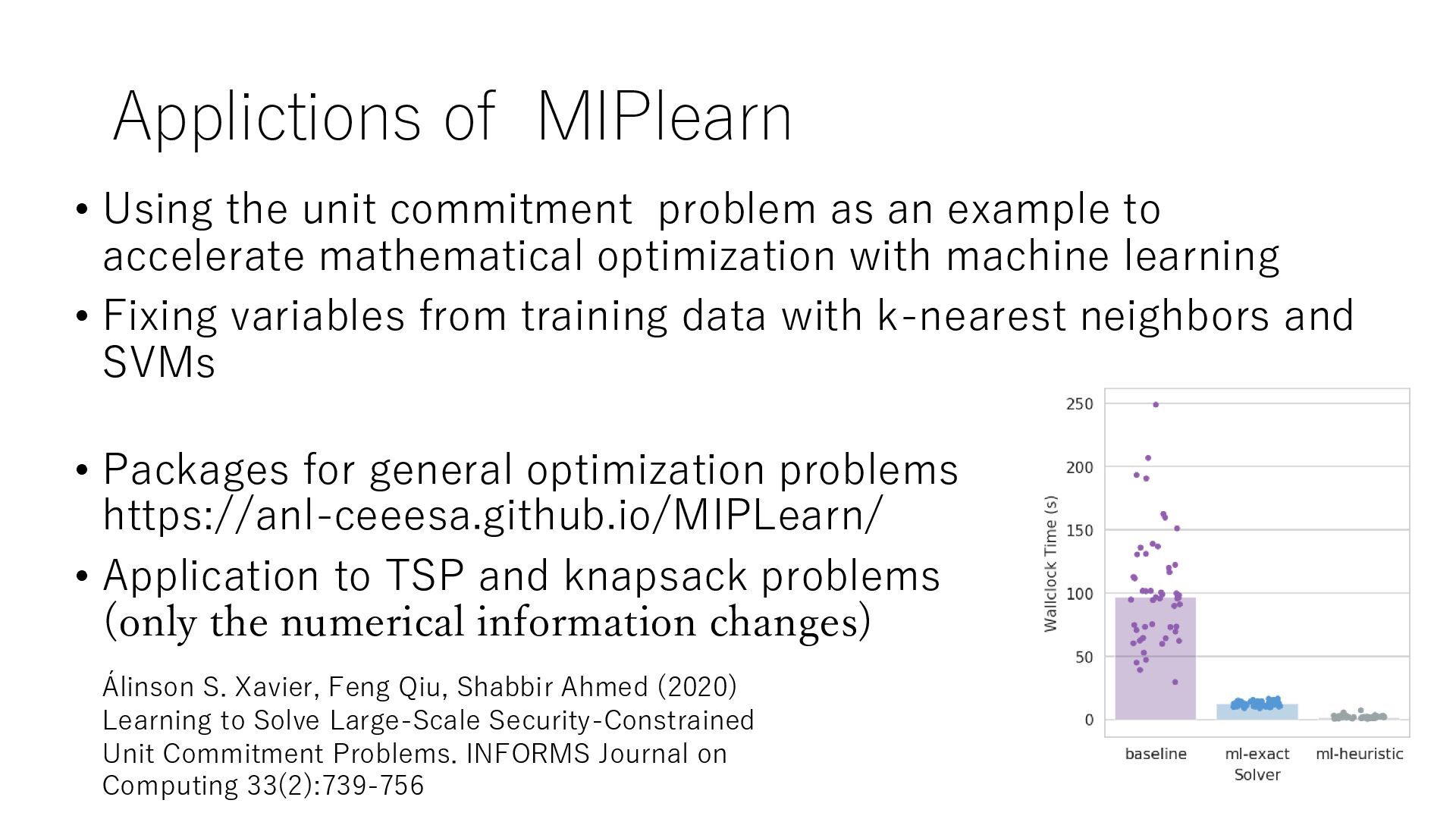
an example to accelerate mathematical optimization with machine learning • Fixing variables from training data with k-nearest neighbors and SVMs • Packages for general optimization problems https://anl-ceeesa.github.io/MIPLearn/ • Application to TSP and knapsack problems (only the numerical information changes) Álinson S. Xavier, Feng Qiu, Shabbir Ahmed (2020) Learning to Solve Large-Scale Security-Constrained Unit Commitment Problems. INFORMS Journal on Computing 33(2):739-756
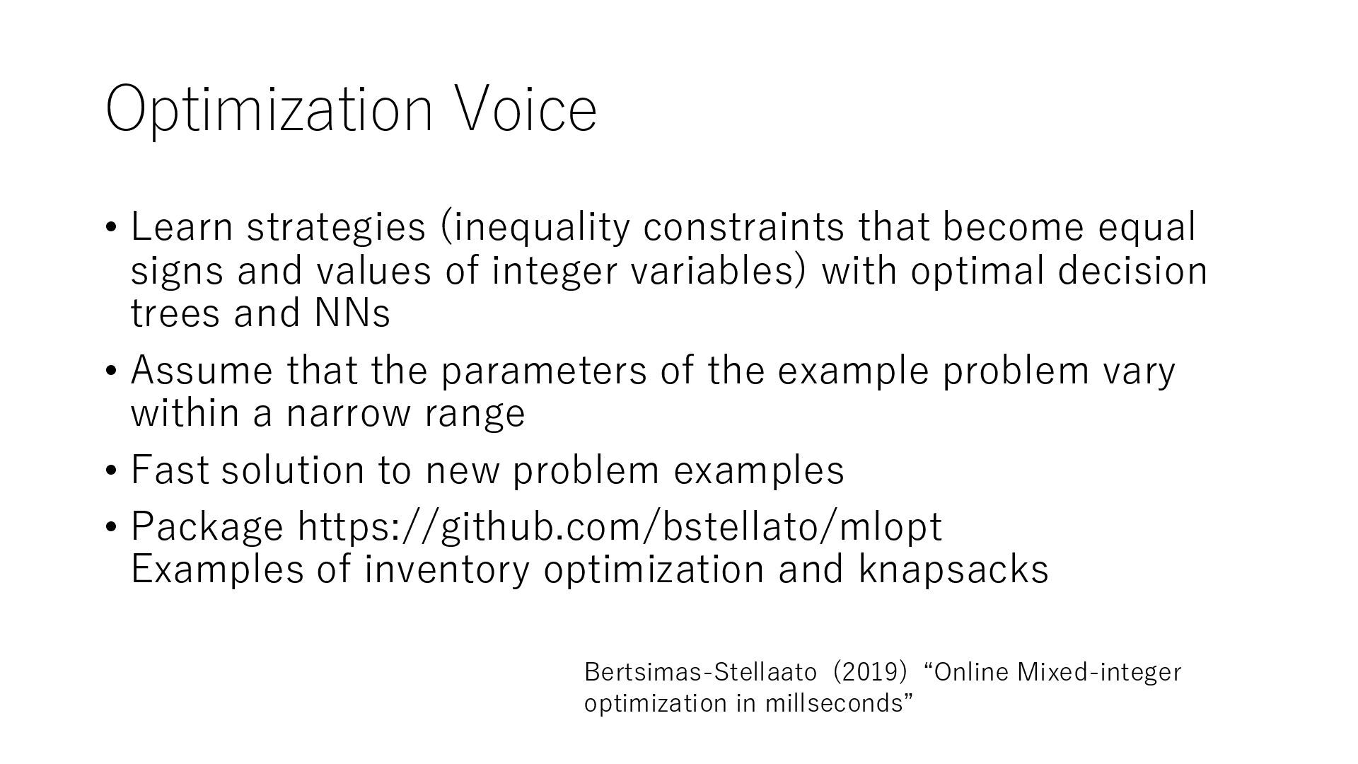
signs and values of integer variables) with optimal decision trees and NNs • Assume that the parameters of the example problem vary within a narrow range • Fast solution to new problem examples • Package https://github.com/bstellato/mlopt Examples of inventory optimization and knapsacks Bertsimas-Stellaato (2019) “Online Mixed-integer optimization in millseconds”
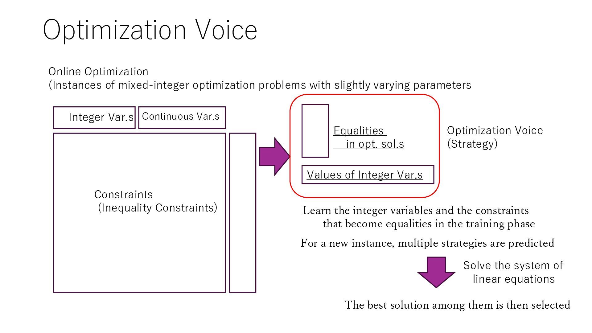
Continuous Var.s 朱 Equalities in opt. sol.s 朱 朱 Values of Integer Var.s Optimization Voice (Strategy) Online Optimization (Instances of mixed-integer optimization problems with slightly varying parameters Learn the integer variables and the constraints that become equalities in the training phase For a new instance, multiple strategies are predicted The best solution among them is then selected Solve the system of linear equations
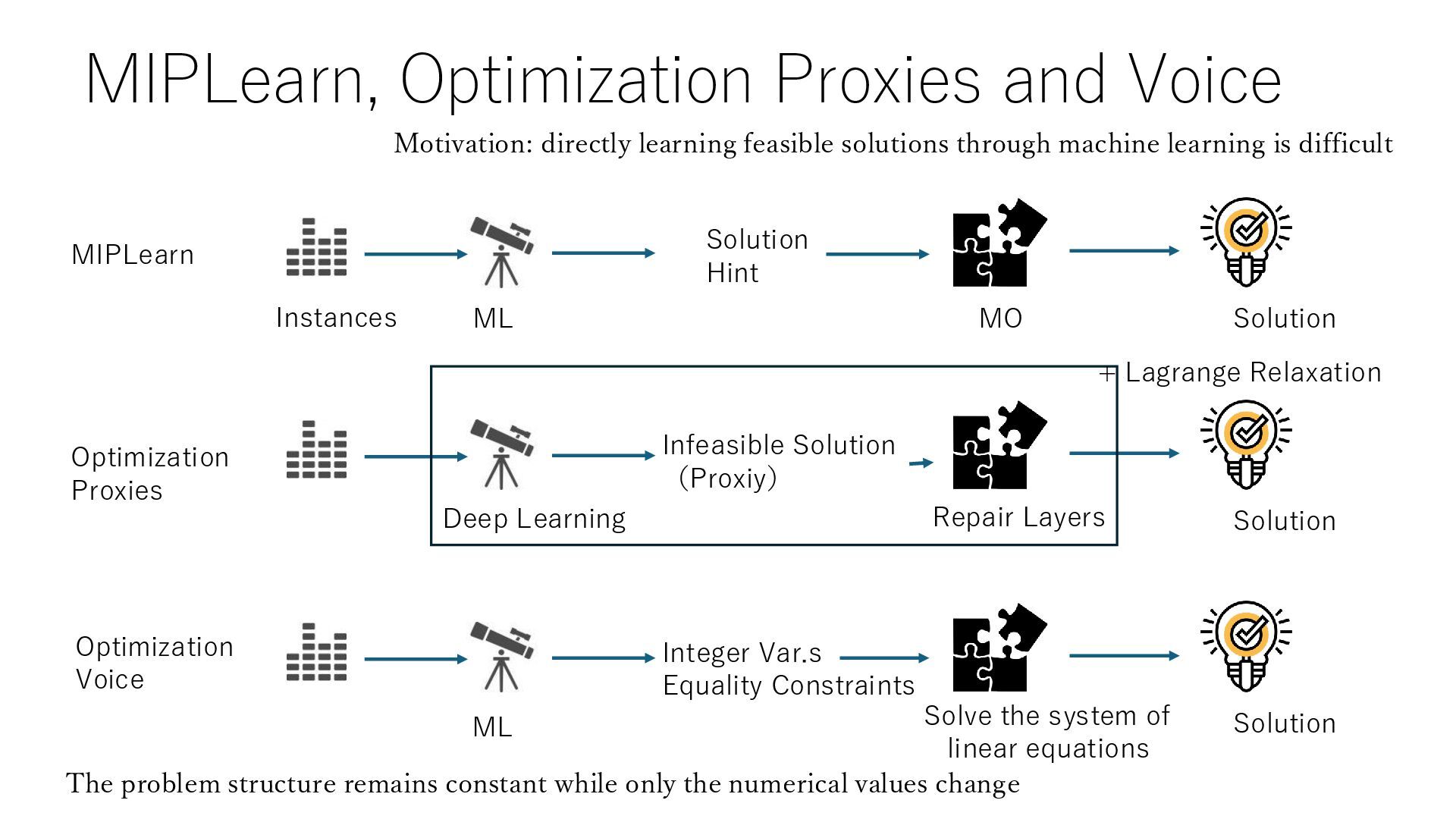
Solution Hint Optimization Proxies Repair Layers Solution Infeasible Solution (Proxiy) ML Solution Integer Var.s Equality Constraints Optimization Voice Deep Learning The problem structure remains constant while only the numerical values change + Lagrange Relaxation Motivation: directly learning feasible solutions through machine learning is difficult Solve the system of linear equations
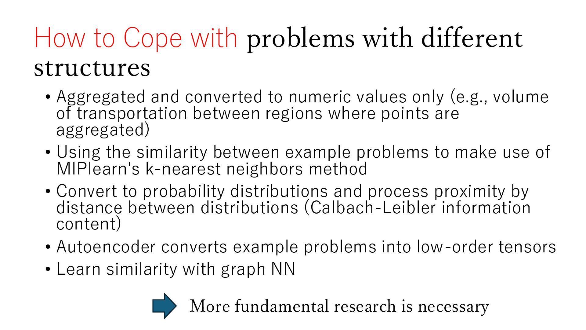
and converted to numeric values only (e.g., volume of transportation between regions where points are aggregated) • Using the similarity between example problems to make use of MIPlearn's k-nearest neighbors method • Convert to probability distributions and process proximity by distance between distributions (Calbach-Leibler information content) • Autoencoder converts example problems into low-order tensors • Learn similarity with graph NN More fundamental research is necessary
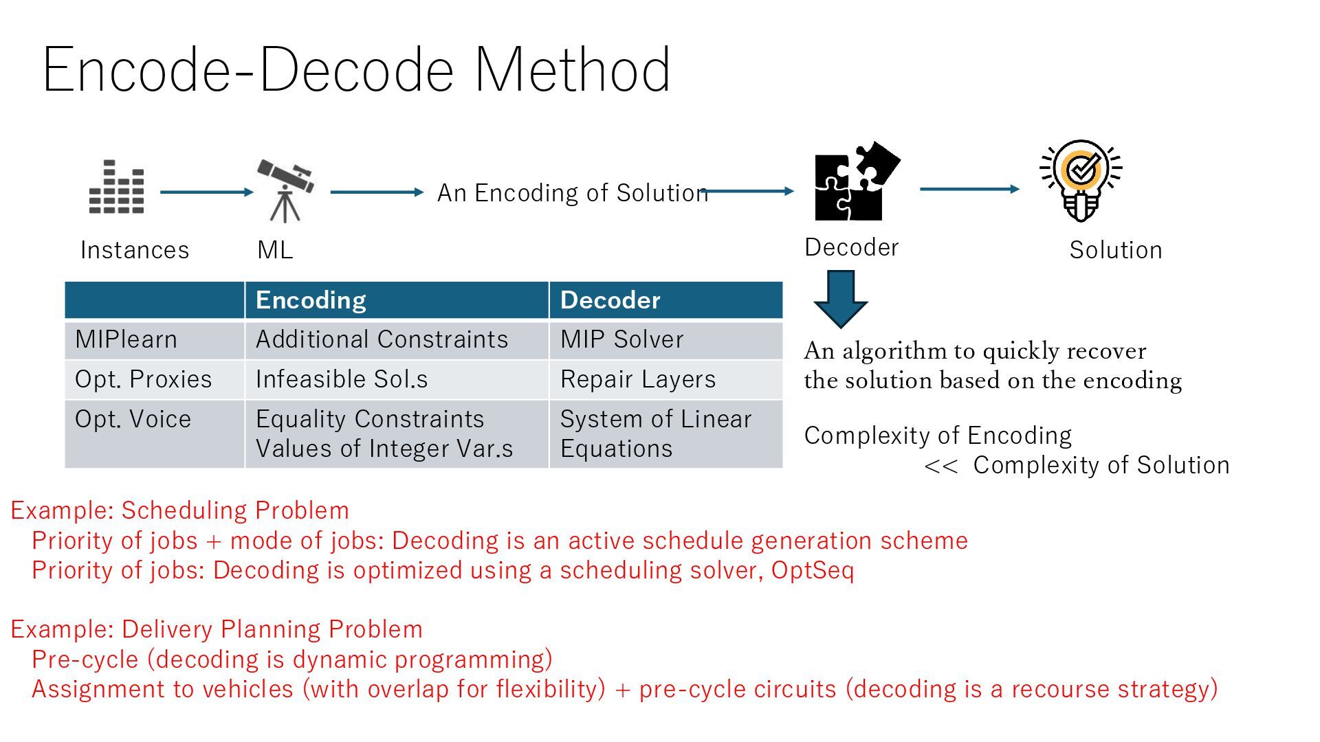
Example: Scheduling Problem Priority of jobs + mode of jobs: Decoding is an active schedule generation scheme Priority of jobs: Decoding is optimized using a scheduling solver, OptSeq Example: Delivery Planning Problem Pre-cycle (decoding is dynamic programming) Assignment to vehicles (with overlap for flexibility) + pre-cycle circuits (decoding is a recourse strategy) An algorithm to quickly recover the solution based on the encoding Encoding Decoder MIPlearn Additional Constraints MIP Solver Opt. Proxies Infeasible Sol.s Repair Layers Opt. Voice Equality Constraints Values of Integer Var.s System of Linear Equations Complexity of Encoding << Complexity of Solution
to be "close" • Useful when the structure of the instances is the same but the numerical value is different. • It is necessary to define ”similarity" of problem instances with different structures. • In many numerical experiments, "similar" problem instances are artificially generated and evaluated. • There are few cases for real-world problems (with the exception of electric power applications)
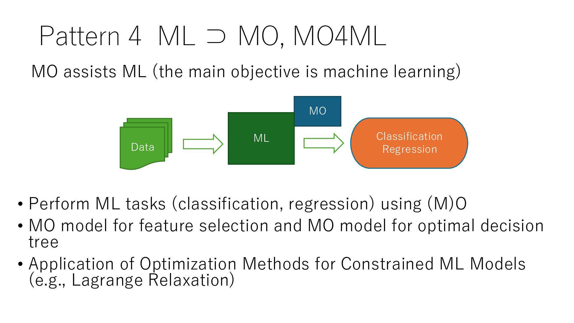
(classification, regression) using (M)O • MO model for feature selection and MO model for optimal decision tree • Application of Optimization Methods for Constrained ML Models (e.g., Lagrange Relaxation) MO Data Classification Regression ML MO assists ML (the main objective is machine learning)
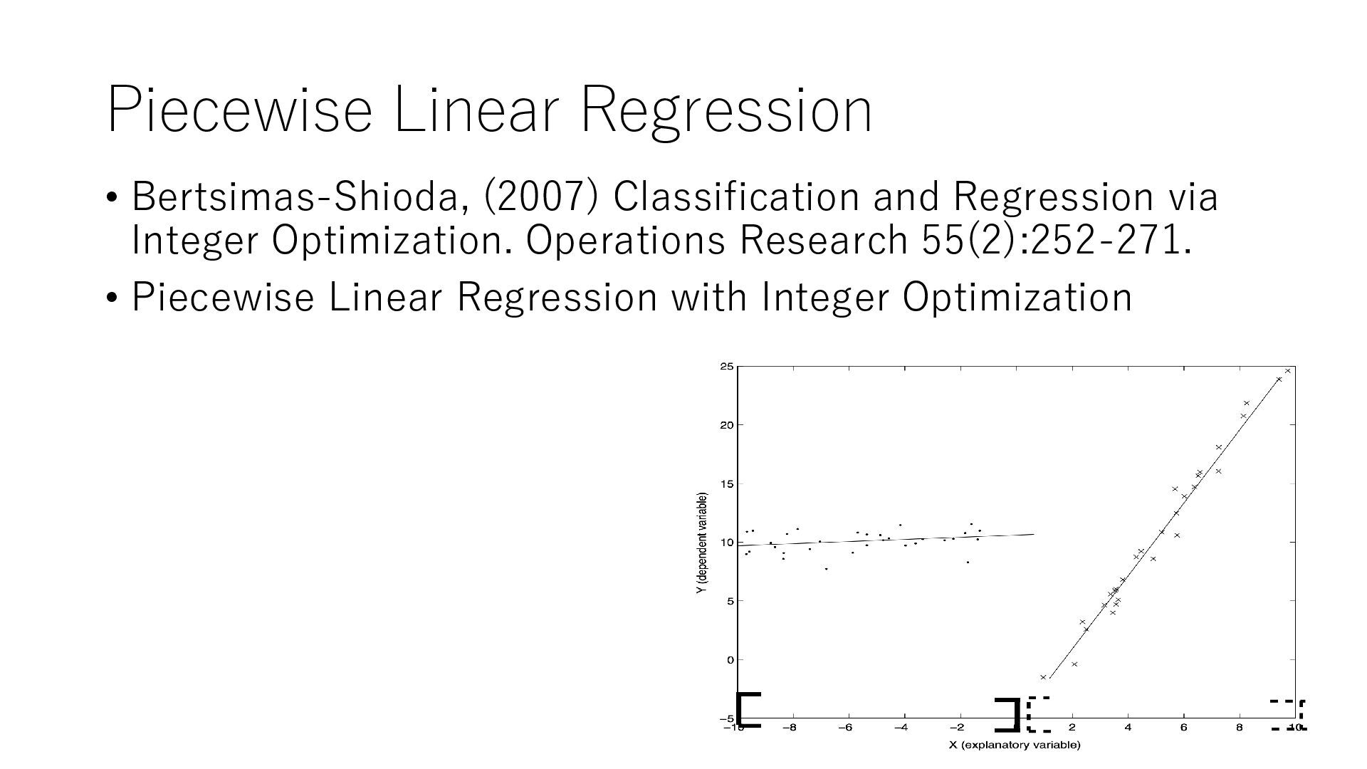
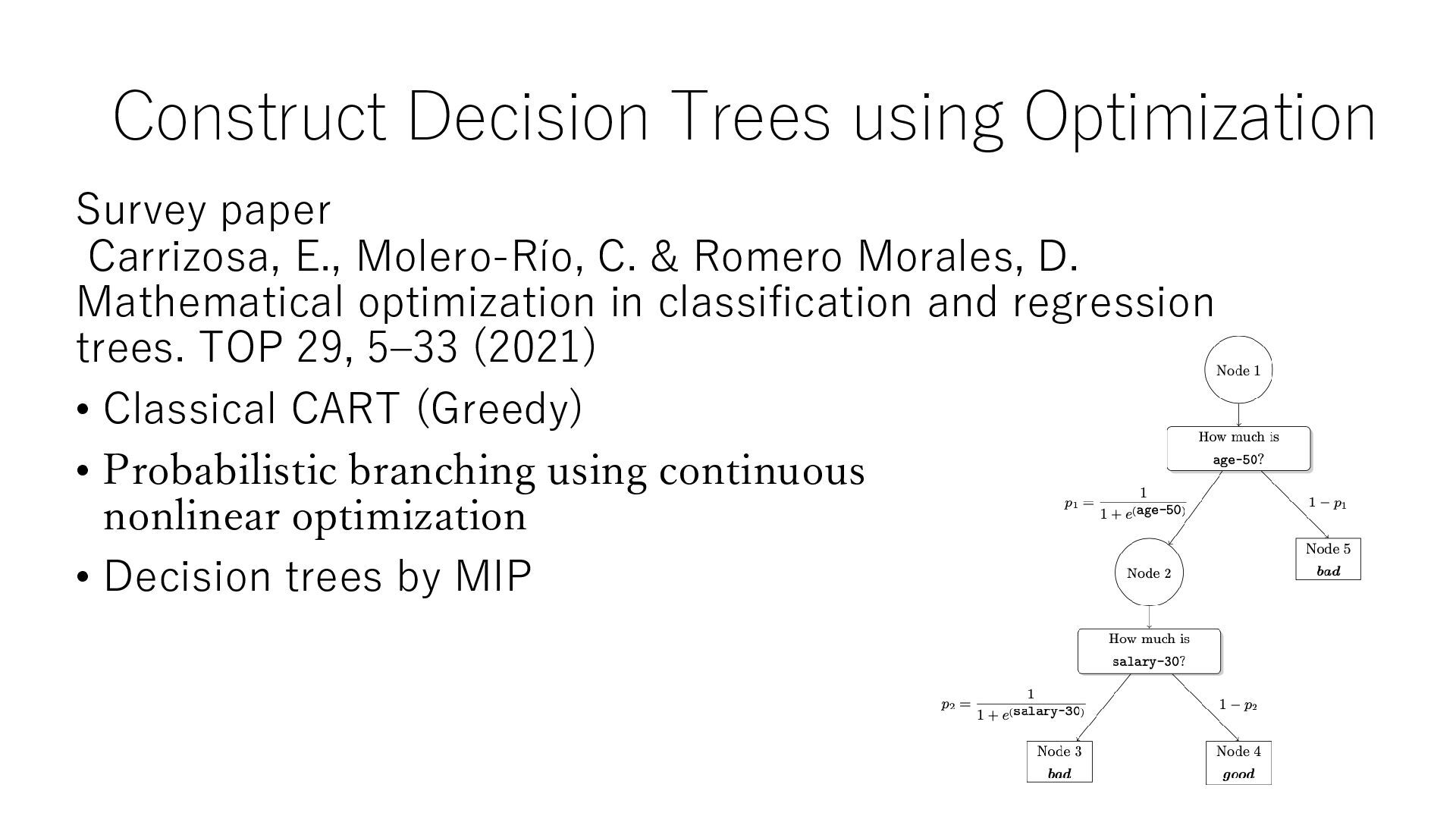
C. & Romero Morales, D. Mathematical optimization in classification and regression trees. TOP 29, 5–33 (2021) • Classical CART (Greedy) • Probabilistic branching using continuous nonlinear optimization • Decision trees by MIP
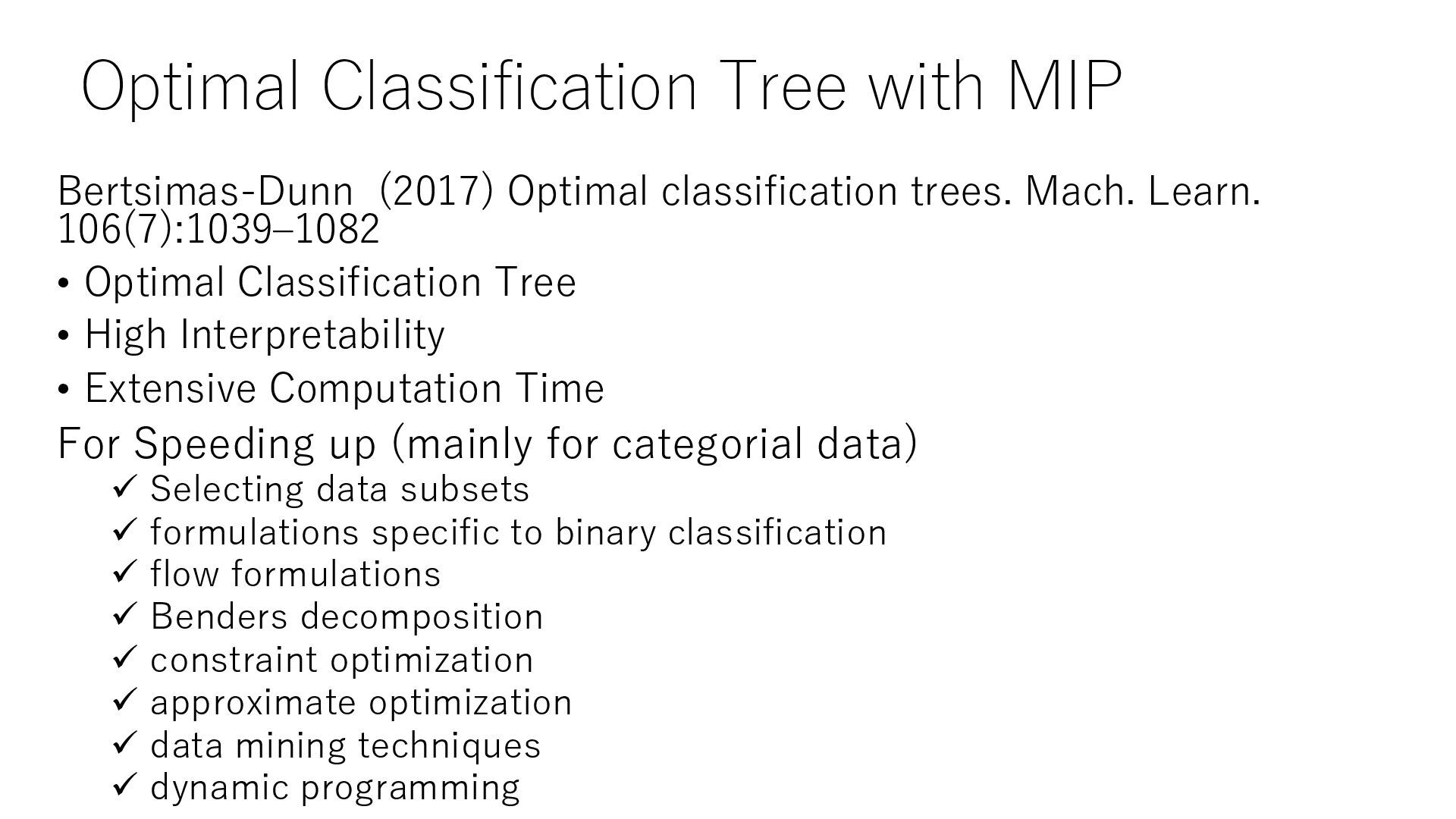
Mach. Learn. 106(7):1039–1082 • Optimal Classification Tree • High Interpretability • Extensive Computation Time For Speeding up (mainly for categorial data) ✓ Selecting data subsets ✓ formulations specific to binary classification ✓ flow formulations ✓ Benders decomposition ✓ constraint optimization ✓ approximate optimization ✓ data mining techniques ✓ dynamic programming
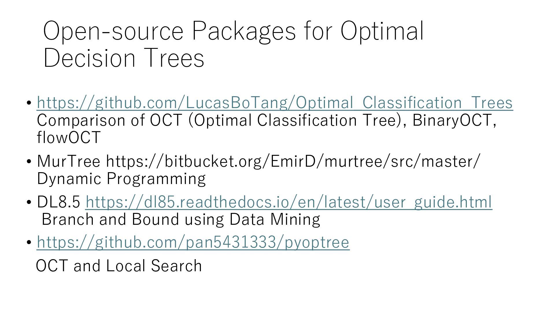
OCT (Optimal Classification Tree), BinaryOCT, flowOCT • MurTree https://bitbucket.org/EmirD/murtree/src/master/ Dynamic Programming • DL8.5 https://dl85.readthedocs.io/en/latest/user_guide.html Branch and Bound using Data Mining • https://github.com/pan5431333/pyoptree OCT and Local Search
learning is a powerful tool when used correctly • Several fast methods have been proposed for categorical data • For continuous data, it is necessary to either apply appropriate discretization or use approximate optimization
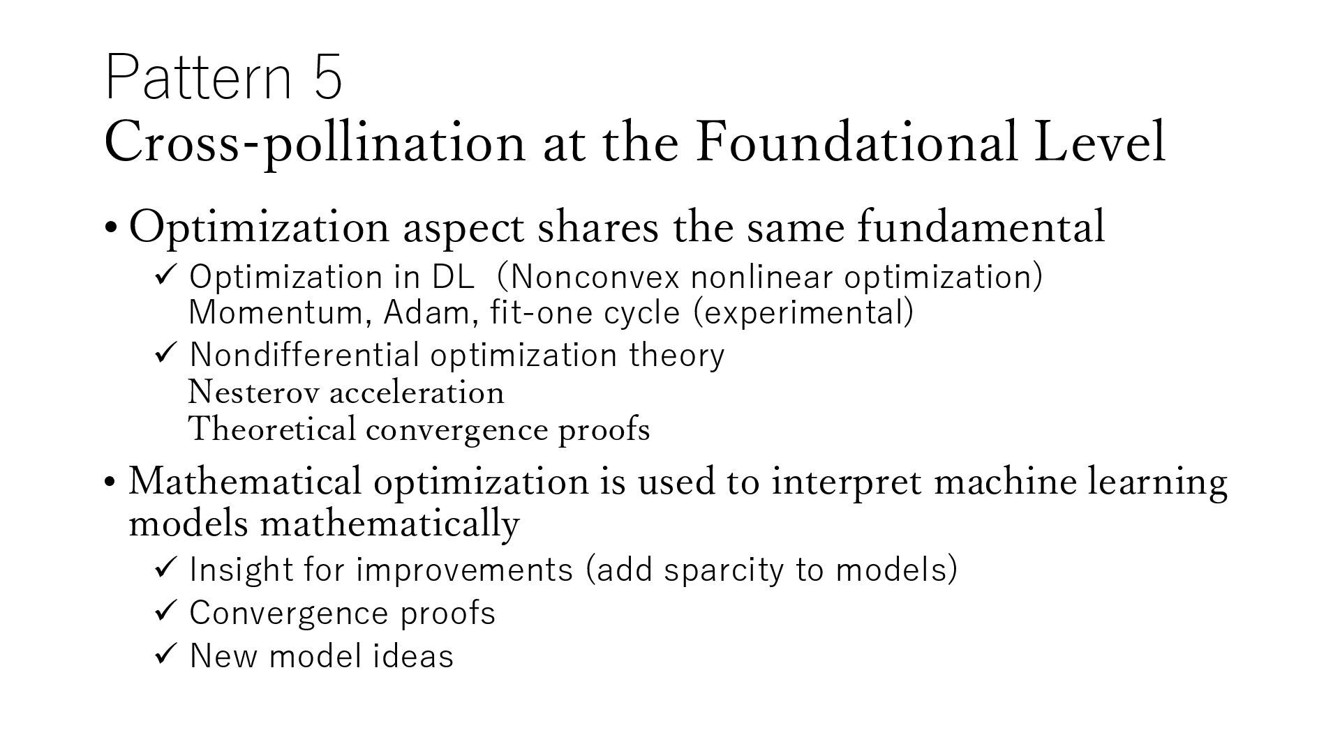
shares the same fundamental ✓ Optimization in DL(Nonconvex nonlinear optimization) Momentum, Adam, fit-one cycle (experimental) ✓ Nondifferential optimization theory Nesterov acceleration Theoretical convergence proofs • Mathematical optimization is used to interpret machine learning models mathematically ✓ Insight for improvements (add sparcity to models) ✓ Convergence proofs ✓ New model ideas
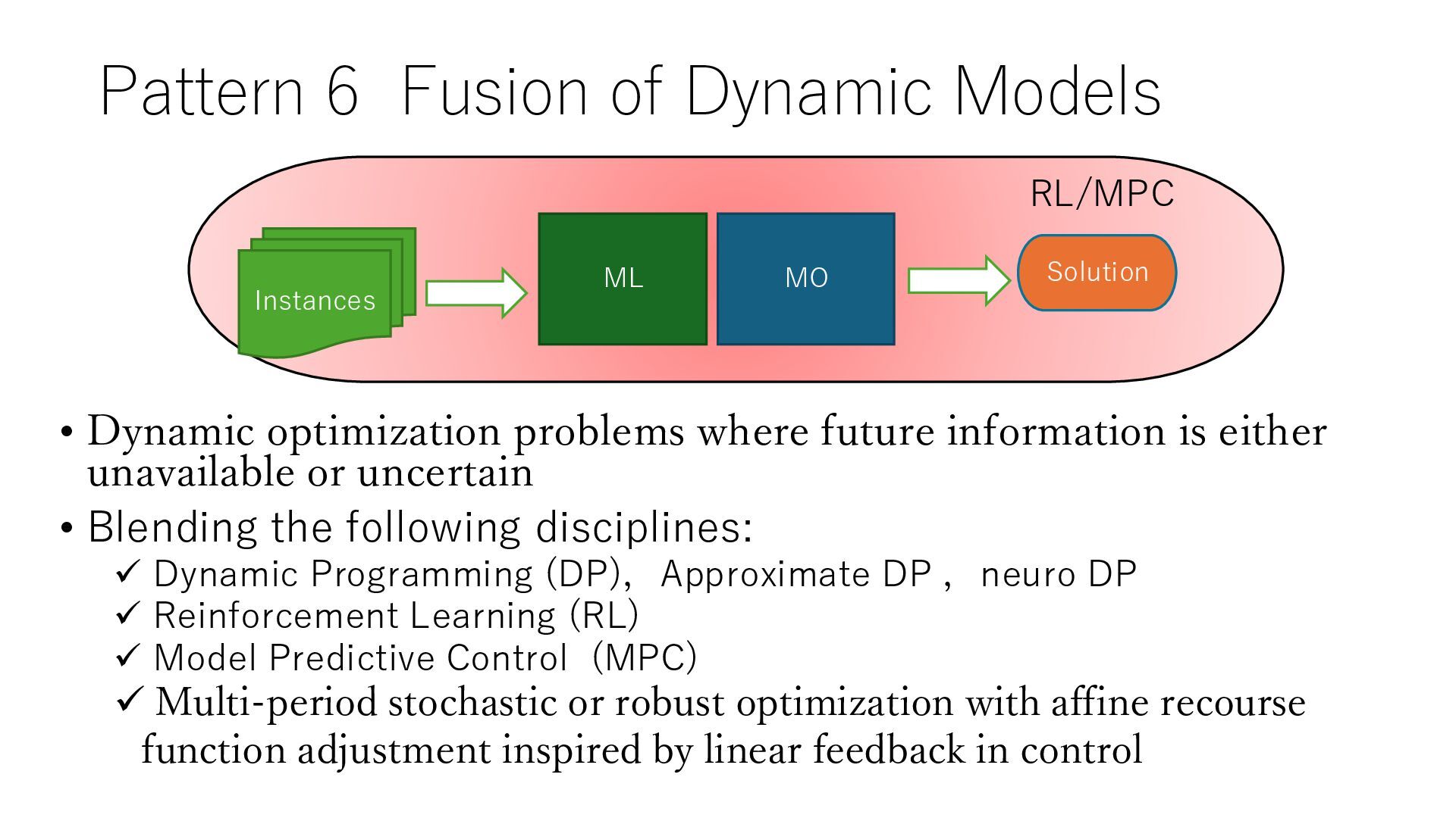
where future information is either unavailable or uncertain • Blending the following disciplines: ✓ Dynamic Programming (DP),Approximate DP ,neuro DP ✓ Reinforcement Learning (RL) ✓ Model Predictive Control (MPC) ✓ Multi-period stochastic or robust optimization with affine recourse function adjustment inspired by linear feedback in control MO Instances Solution ML RL/MPC
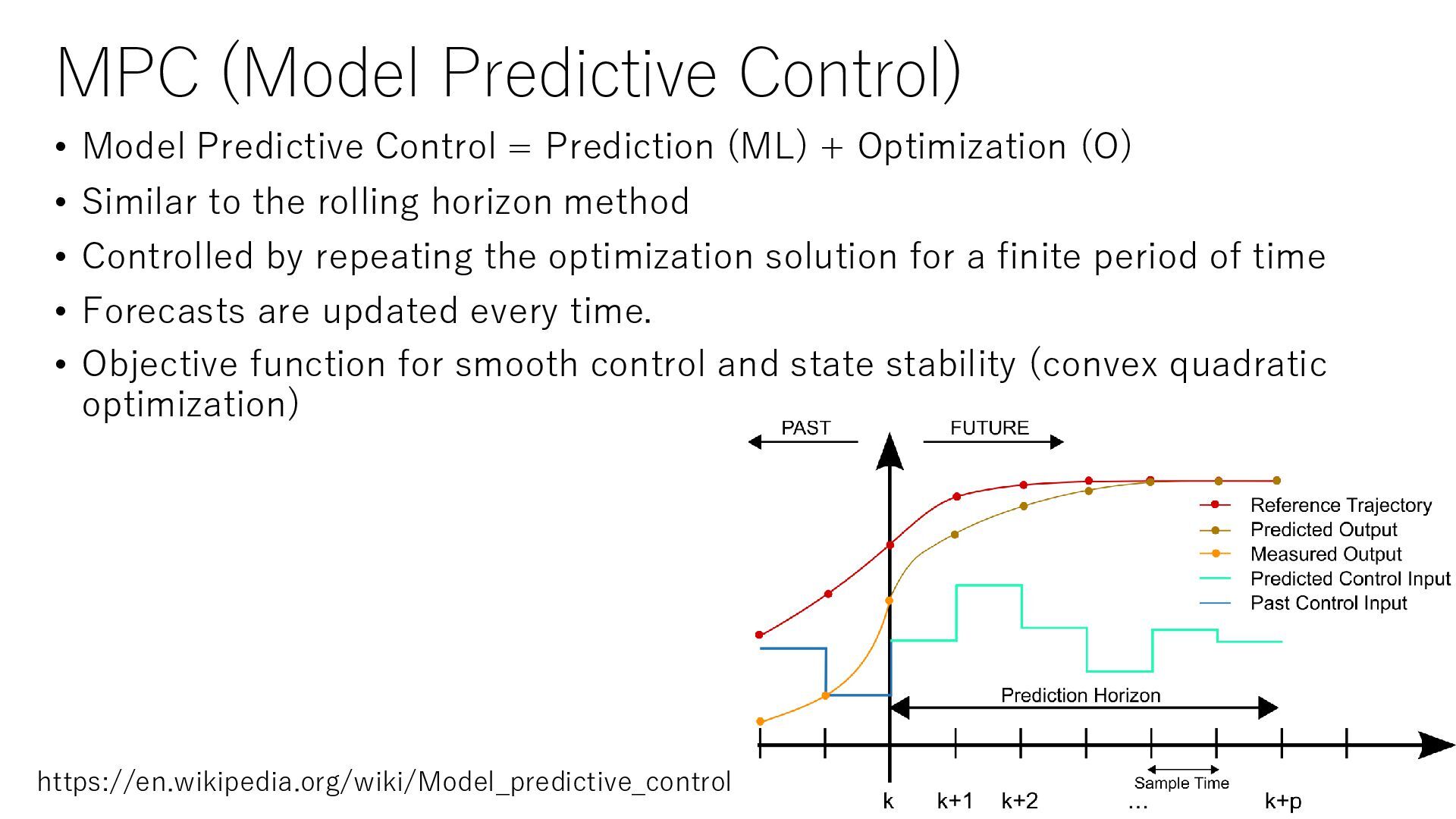
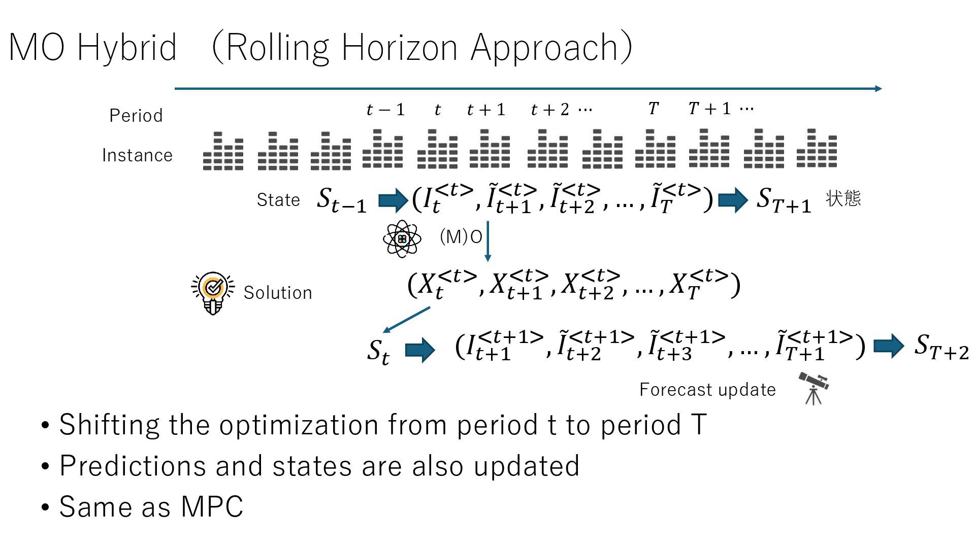
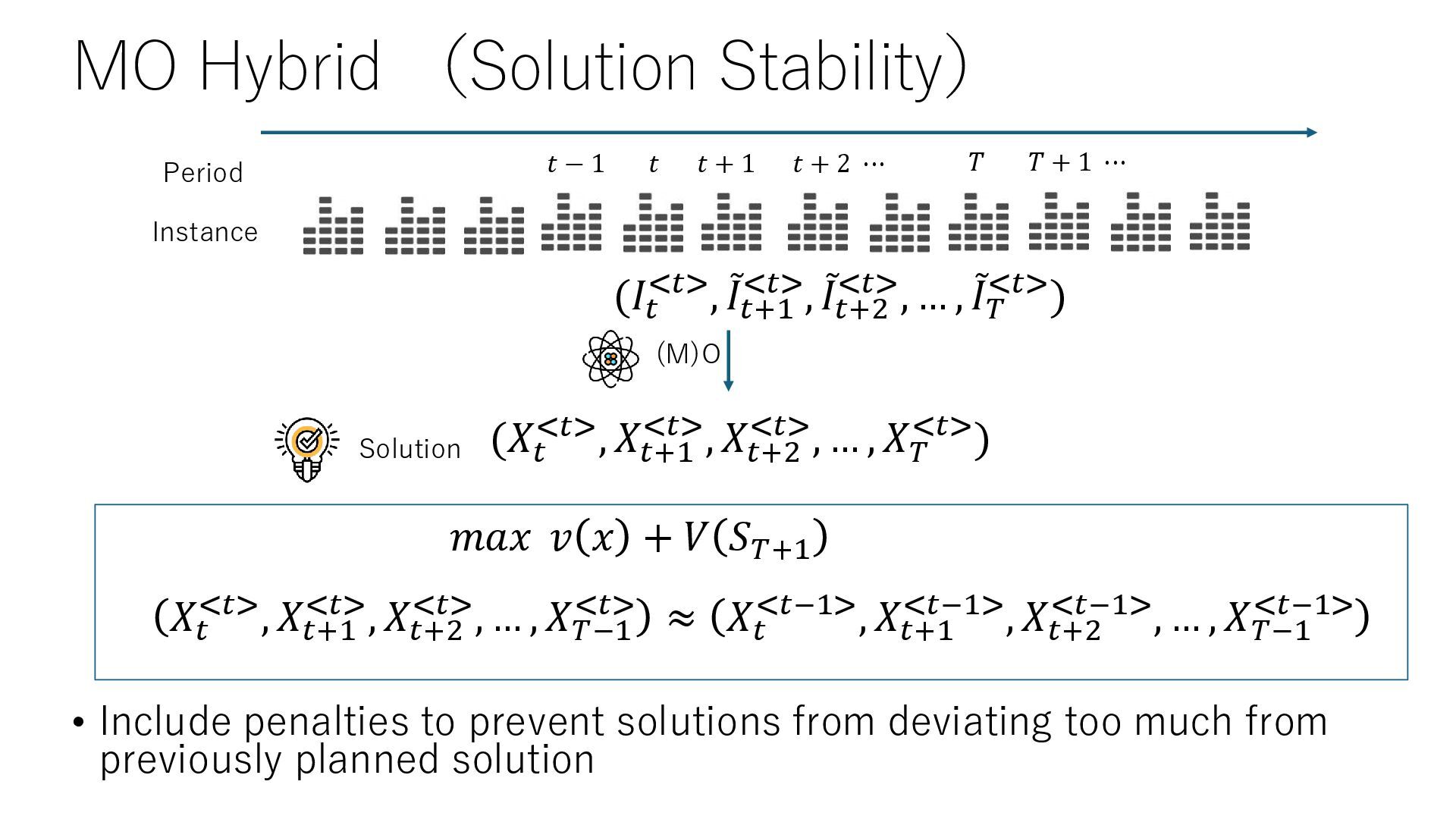
(ML) + Optimization (O) • Similar to the rolling horizon method • Controlled by repeating the optimization solution for a finite period of time • Forecasts are updated every time. • Objective function for smooth control and state stability (convex quadratic optimization) https://en.wikipedia.org/wiki/Model_predictive_control
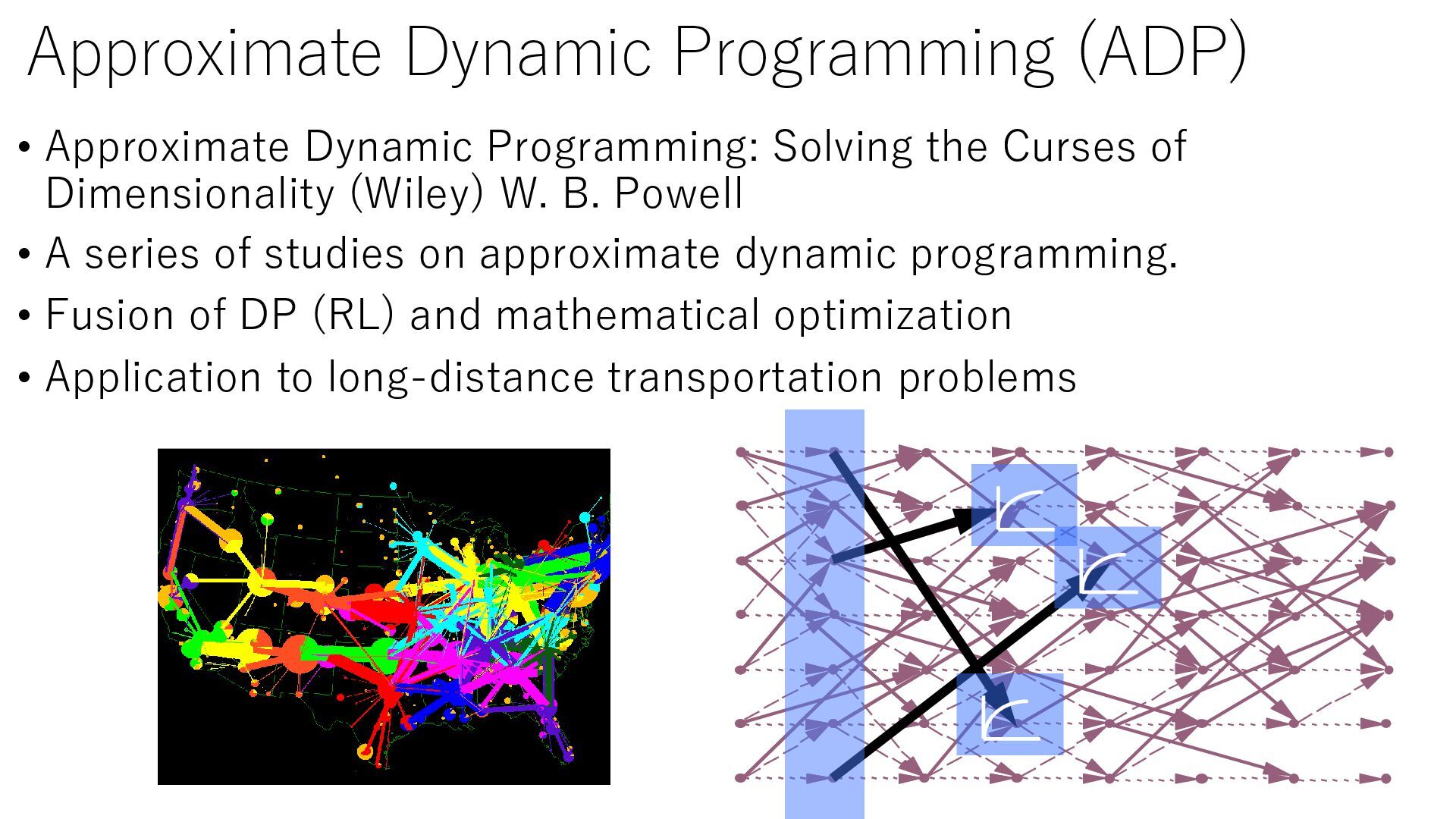
Curses of Dimensionality (Wiley) W. B. Powell • A series of studies on approximate dynamic programming. • Fusion of DP (RL) and mathematical optimization • Application to long-distance transportation problems
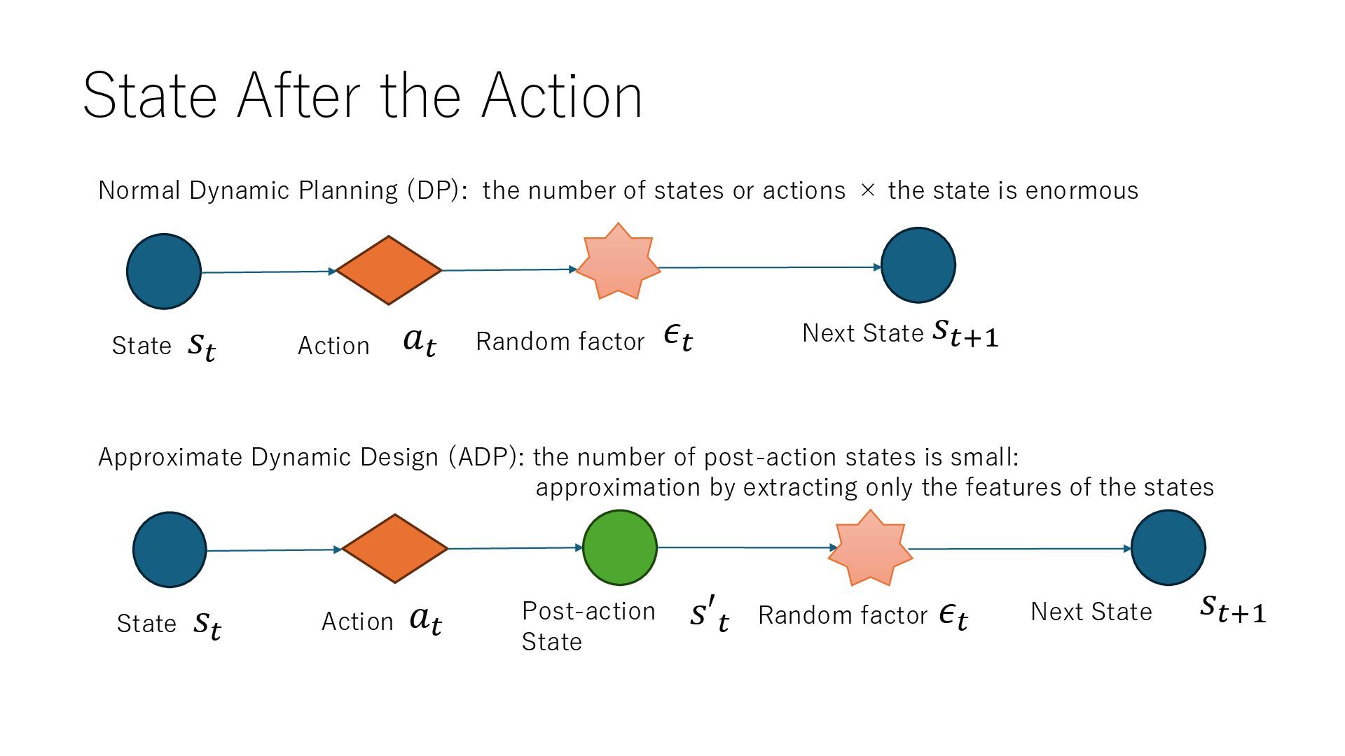
𝑠𝑡 𝑎𝑡 𝑠′𝑡 𝑠𝑡+1 Random factor 𝜖𝑡 State Action Next State 𝑠𝑡 𝑎𝑡 𝑠𝑡+1 Random factor 𝜖𝑡 Normal Dynamic Planning (DP): the number of states or actions × the state is enormous Approximate Dynamic Design (ADP): the number of post-action states is small: approximation by extracting only the features of the states
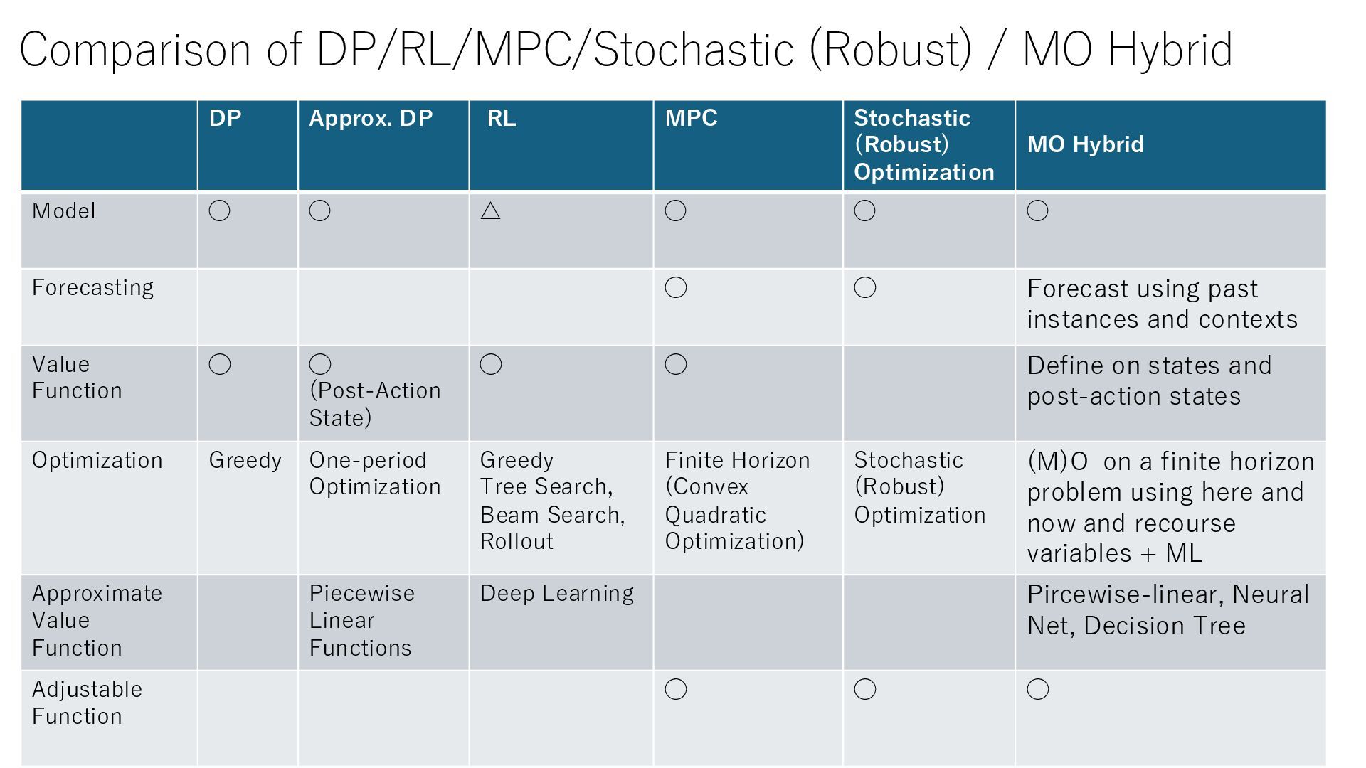
RL MPC Stochastic (Robust) Optimization MO Hybrid Model ◯ ◯ △ ◯ ◯ ◯ Forecasting ◯ ◯ Forecast using past instances and contexts Value Function ◯ ◯ (Post-Action State) ◯ ◯ Define on states and post-action states Optimization Greedy One-period Optimization Greedy Tree Search, Beam Search, Rollout Finite Horizon (Convex Quadratic Optimization) Stochastic (Robust) Optimization (M)O on a finite horizon problem using here and now and recourse variables + ML Approximate Value Function Piecewise Linear Functions Deep Learning Pircewise-linear, Neural Net, Decision Tree Adjustable Function ◯ ◯ ◯
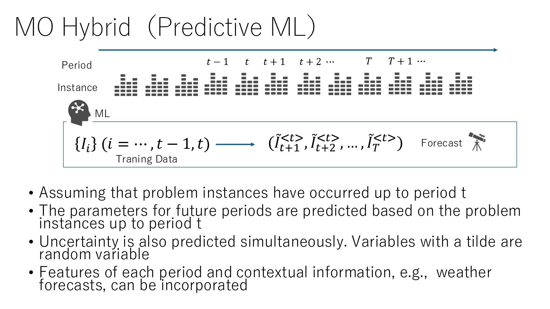
up to period t • The parameters for future periods are predicted based on the problem instances up to period t • Uncertainty is also predicted simultaneously. Variables with a tilde are random variable • Features of each period and contextual information, e.g., weather forecasts, can be incorporated Forecast Traning Data Period Instance 𝑡 − 1 𝑡 𝑡 + 1 𝑡 + 2 ⋯ 𝑇 𝑇 + 1 ⋯ ML 𝐼𝑖 (𝑖 = ⋯ , 𝑡 − 1, 𝑡) (ሚ 𝐼𝑡+1 <𝑡>, ሚ 𝐼𝑡+2 <𝑡>, … , ሚ 𝐼𝑇 <𝑡>)
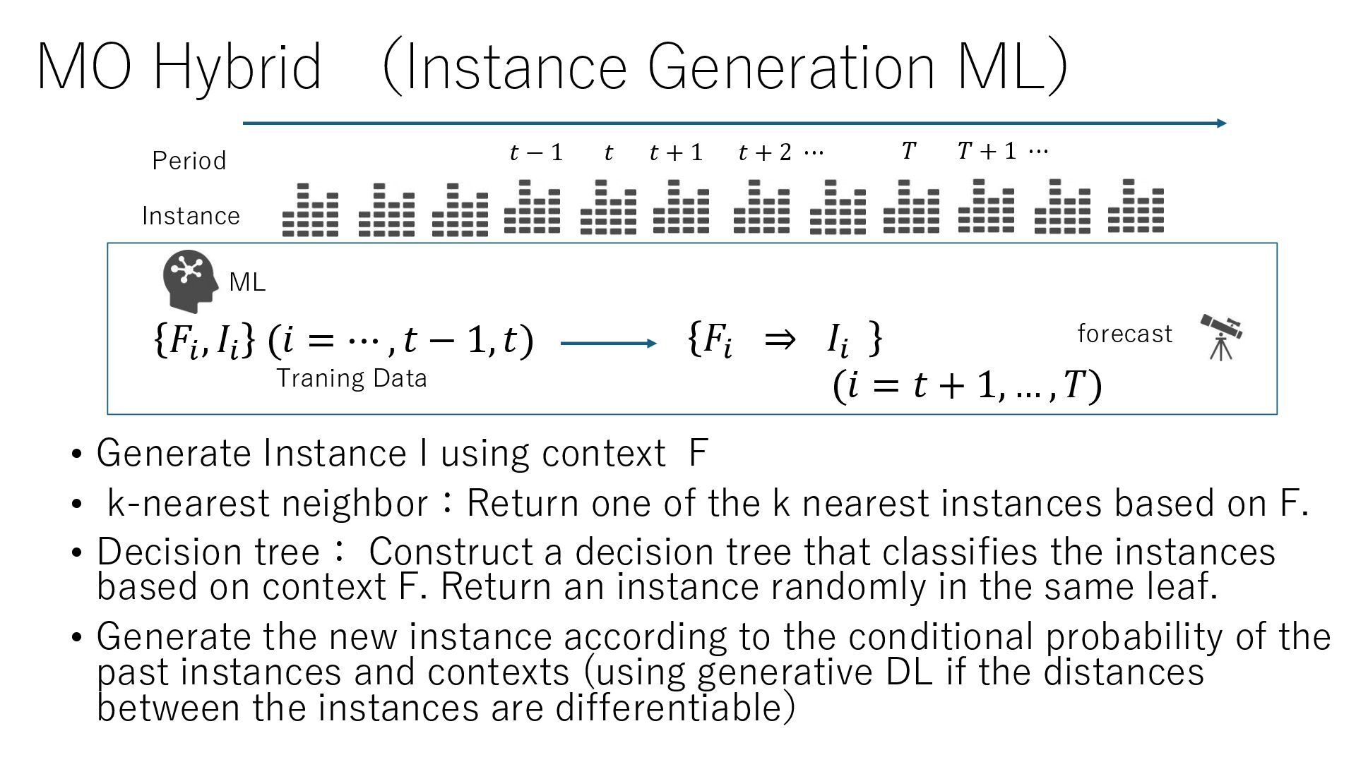
context F • k-nearest neighbor:Return one of the k nearest instances based on F. • Decision tree: Construct a decision tree that classifies the instances based on context F. Return an instance randomly in the same leaf. • Generate the new instance according to the conditional probability of the past instances and contexts (using generative DL if the distances between the instances are differentiable) forecast Traning Data Period Instance 𝑡 − 1 𝑡 𝑡 + 1 𝑡 + 2 ⋯ 𝑇 𝑇 + 1 ⋯ ML 𝐹𝑖 , 𝐼𝑖 (𝑖 = ⋯ , 𝑡 − 1, 𝑡) 𝐹𝑖 ⇒ 𝐼𝑖 (𝑖 = 𝑡 + 1, … , 𝑇)
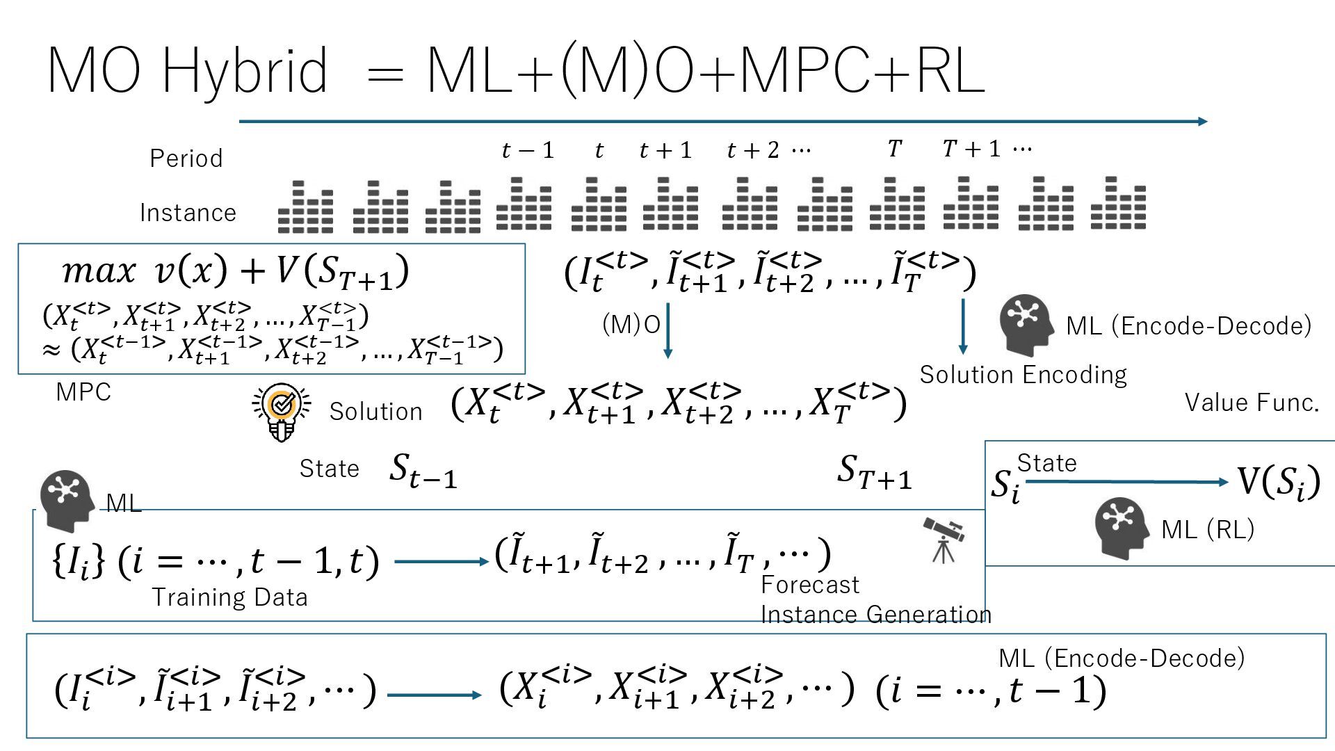
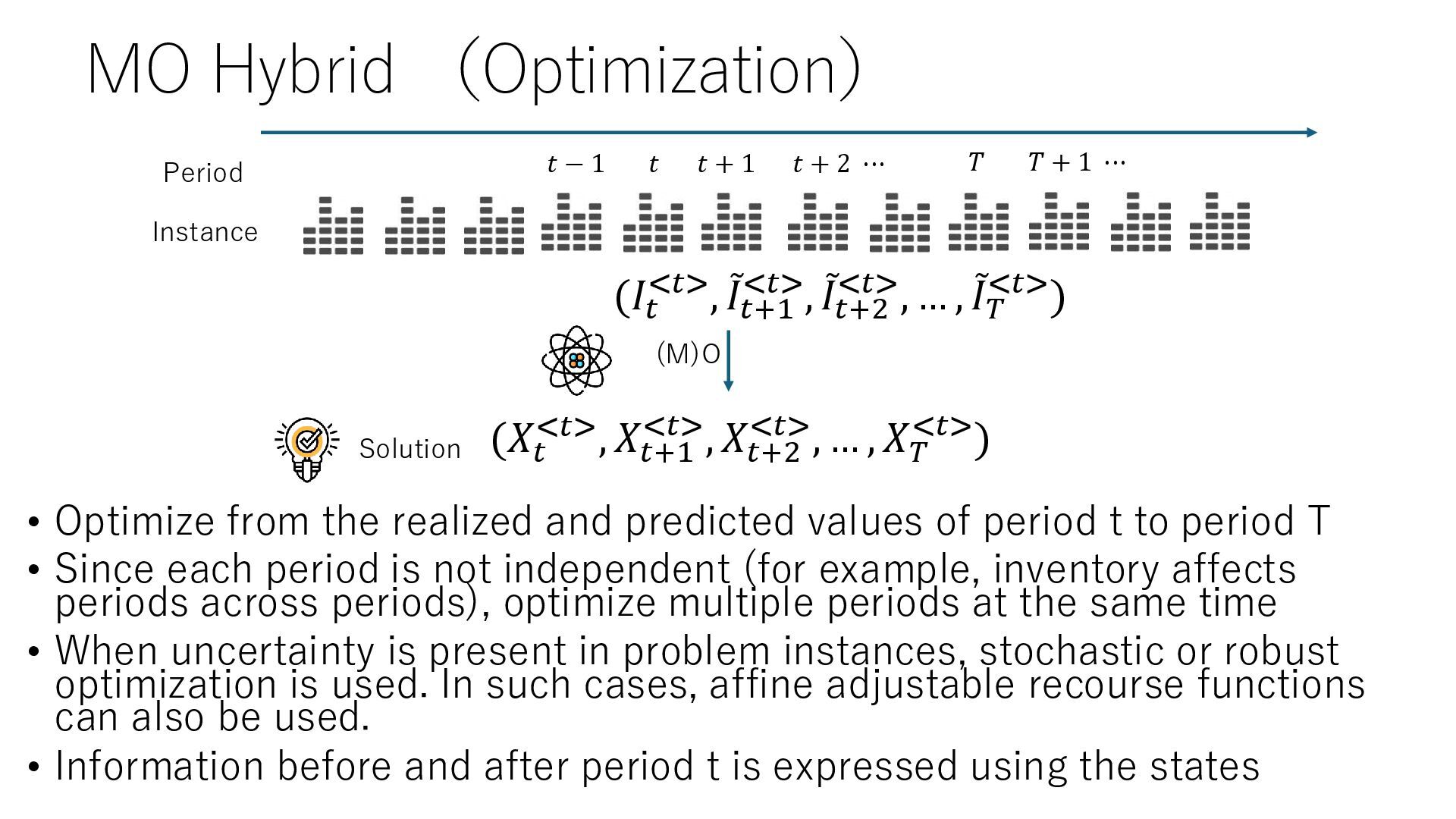
values of period t to period T • Since each period is not independent (for example, inventory affects periods across periods), optimize multiple periods at the same time • When uncertainty is present in problem instances, stochastic or robust optimization is used. In such cases, affine adjustable recourse functions can also be used. • Information before and after period t is expressed using the states (M)O Solution Period Instance 𝑡 − 1 𝑡 𝑡 + 1 𝑡 + 2 ⋯ 𝑇 𝑇 + 1 ⋯ (𝐼𝑡 <𝑡>, ሚ 𝐼𝑡+1 <𝑡>, ሚ 𝐼𝑡+2 <𝑡>, … , ሚ 𝐼𝑇 <𝑡>) (𝑋𝑡 <𝑡>, 𝑋𝑡+1 <𝑡>, 𝑋𝑡+2 <𝑡>, … , 𝑋𝑇 <𝑡>)
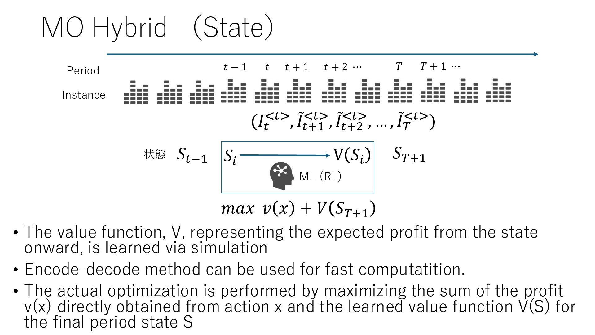
expected profit from the state onward, is learned via simulation • Encode-decode method can be used for fast computatition. • The actual optimization is performed by maximizing the sum of the profit v(x) directly obtained from action x and the learned value function V(S) for the final period state S Period Instance 𝑡 − 1 𝑡 𝑡 + 1 𝑡 + 2 ⋯ 𝑇 𝑇 + 1 ⋯ (𝐼𝑡 <𝑡>, ሚ 𝐼𝑡+1 <𝑡>, ሚ 𝐼𝑡+2 <𝑡>, … , ሚ 𝐼𝑇 <𝑡>) 𝑆𝑡−1 𝑆𝑖 ML (RL) V 𝑆𝑖 𝑆𝑇+1 𝑚𝑎𝑥 𝑣 𝑥 + 𝑉 𝑆𝑇+1 状態
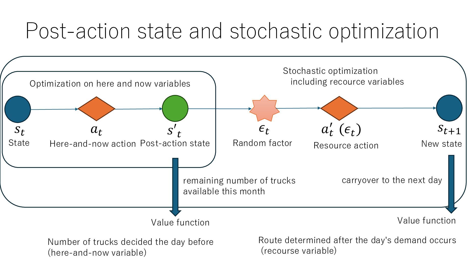
New state 𝑠𝑡 𝑎𝑡 𝑠′𝑡 𝑠𝑡+1 Random factor 𝜖𝑡 Resource action 𝑎𝑡 ′ (𝜖𝑡 ) Optimization on here and now variables Stochastic optimization including recource variables Value function Number of trucks decided the day before (here-and-now variable) Route determined after the day's demand occurs (recourse variable) remaining number of trucks available this month carryover to the next day Value function
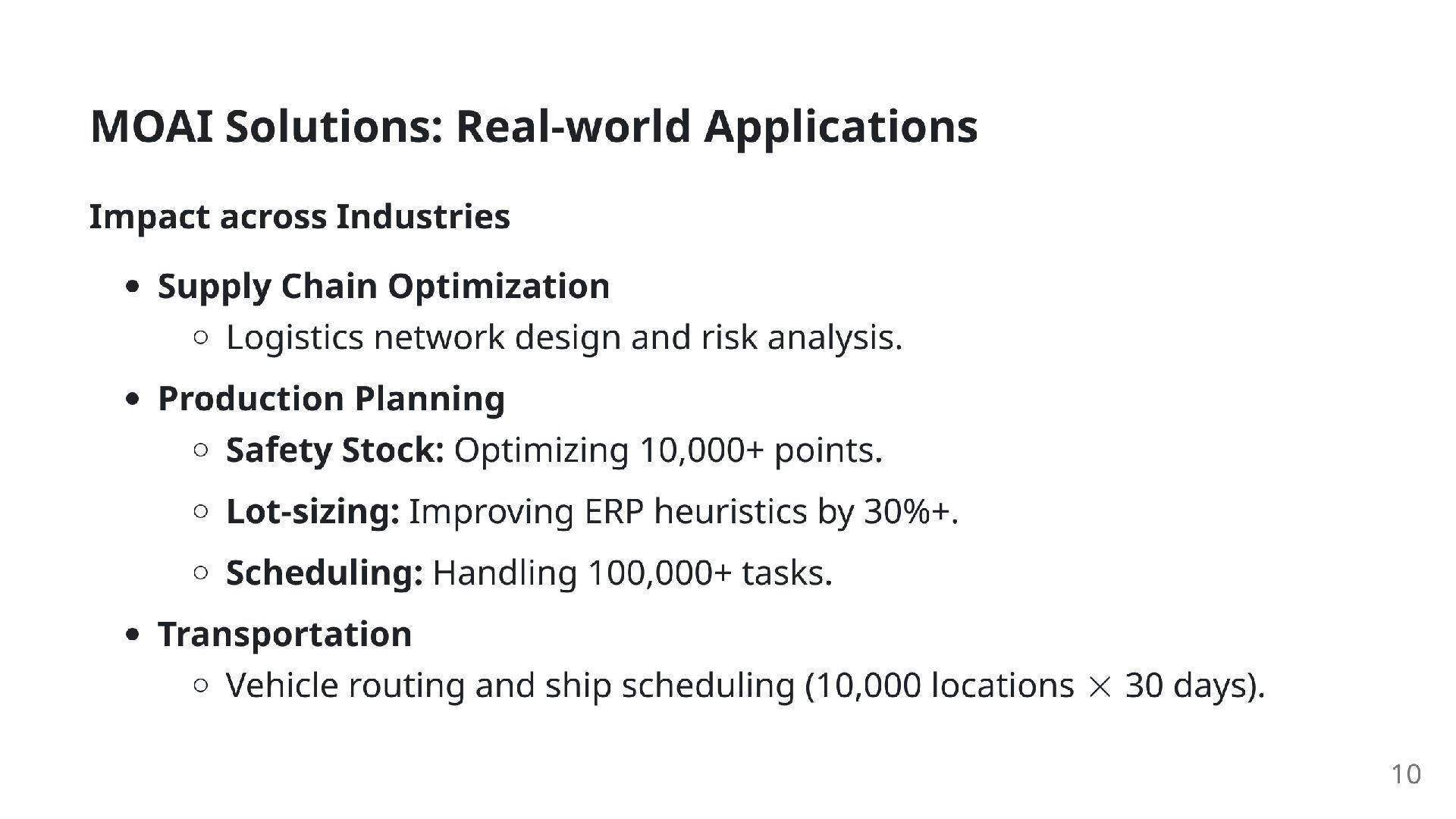
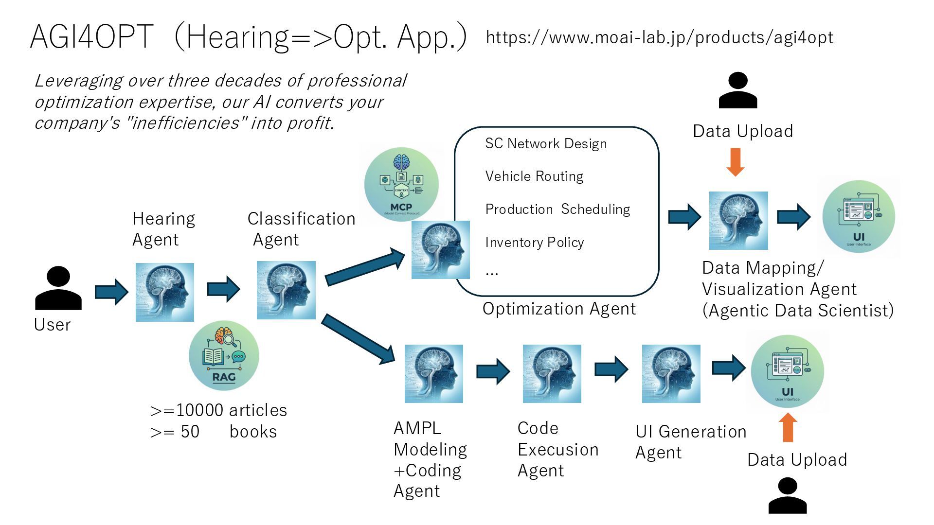
Production Scheduling Inventory Policy … Hearing Agent AMPL Modeling +Coding Agent Code Execusion Agent https://www.moai-lab.jp/products/agi4opt >=10000 articles >= 50 books Optimization Agent Data Mapping/ Visualization Agent (Agentic Data Scientist) UI Generation Agent Data Upload Data Upload Leveraging over three decades of professional optimization expertise, our AI converts your company's "inefficiencies" into profit.
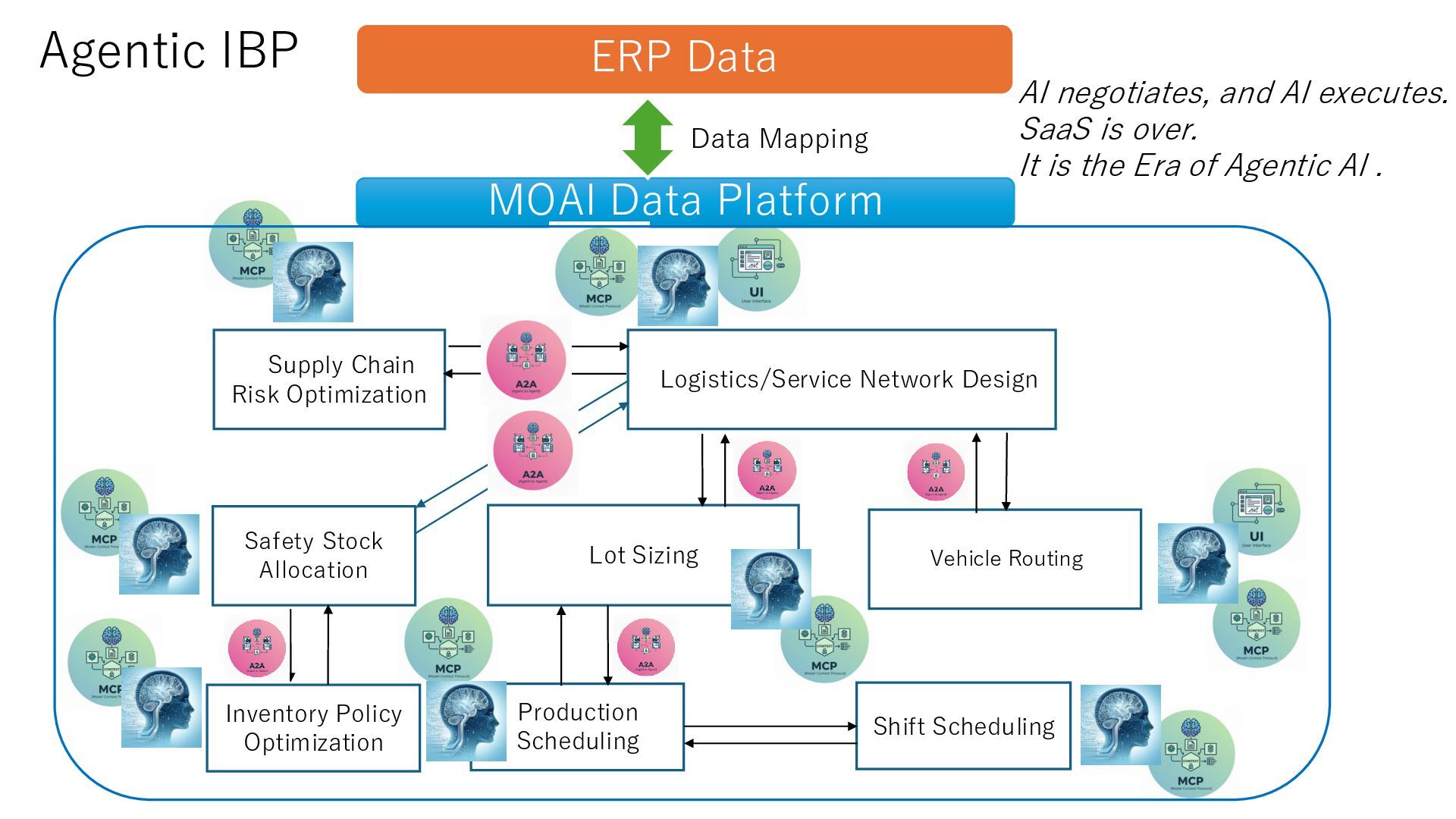
Sizing Logistics/Service Network Design Vehicle Routing Supply Chain Risk Optimization Stage BOM Safety Stock Allocation Inventory Policy Optimization Shift Scheduling AI negotiates, and AI executes. SaaS is over. It is the Era of Agentic AI . Data Mapping