Bayesian Statistical Analysis: A Gentle Introduction

Get to know the Reverend Bayes.Reverend

Transcript

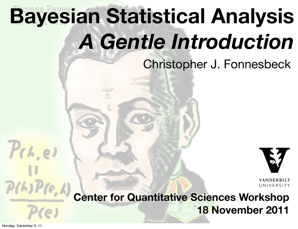
1. Bayesian Statistical Analysis A Gentle Introduction Center for Quantitative Sciences Workshop 18 November 2011 Christopher J. Fonnesbeck Monday, December 5, 11
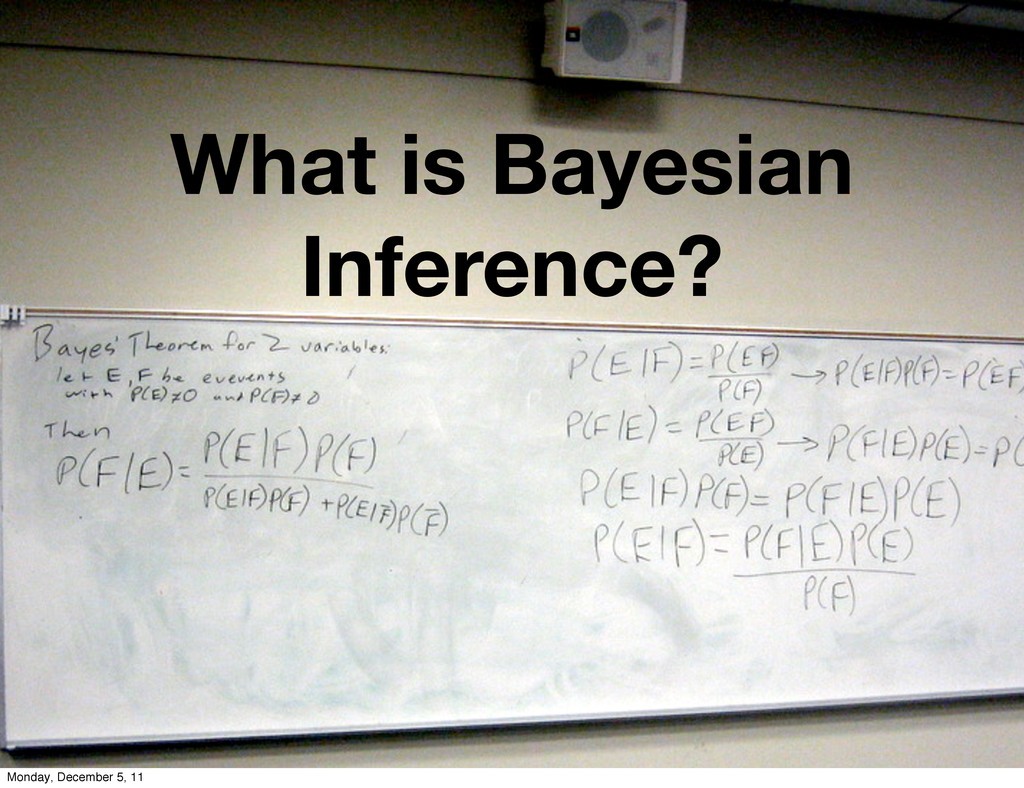
2. What is Bayesian Inference? Monday, December 5, 11
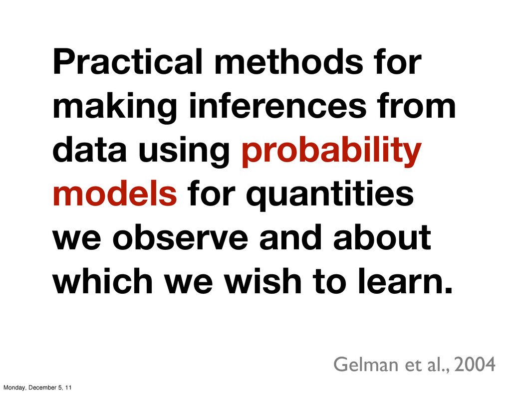
3. Practical methods for making inferences from data using probability models for quantities we observe and about which we wish to learn. Gelman et al., 2004 Monday, December 5, 11
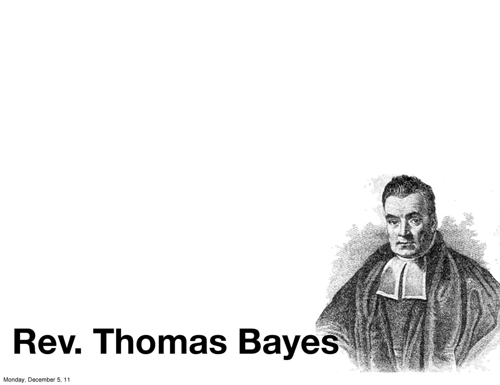
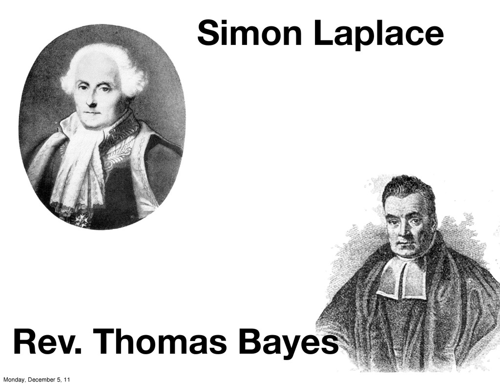
4. Rev. Thomas Bayes Monday, December 5, 11
5. Rev. Thomas Bayes Simon Laplace Monday, December 5, 11
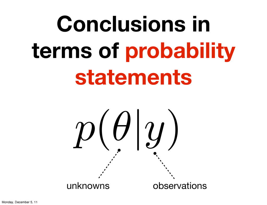
6. Conclusions in terms of probability statements p( |y) unknowns observations Monday, December 5, 11
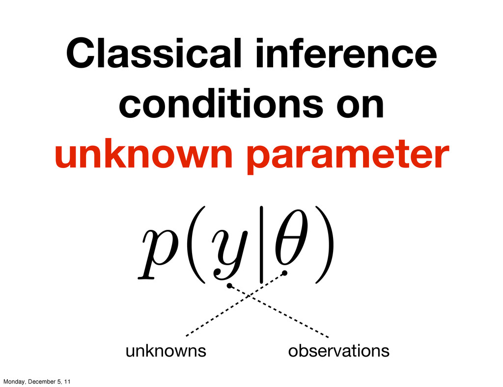
7. Classical inference conditions on unknown parameter p(y| ) unknowns observations Monday, December 5, 11
8. Classical vs Bayesian Statistics Monday, December 5, 11
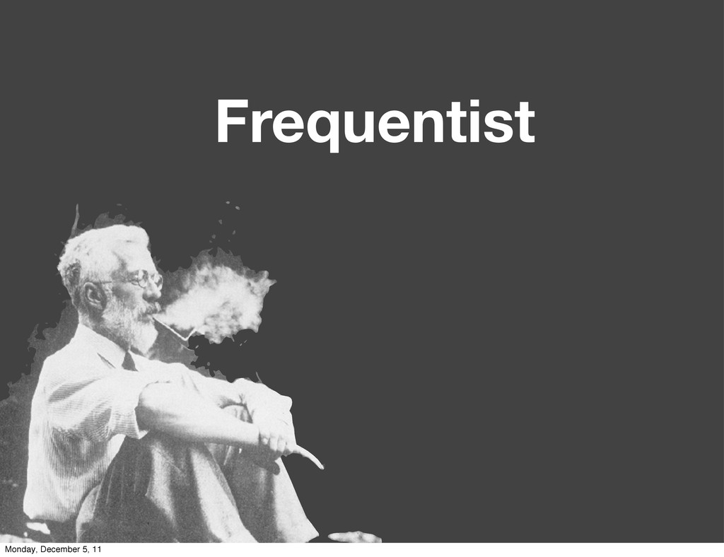
9. Frequentist Monday, December 5, 11
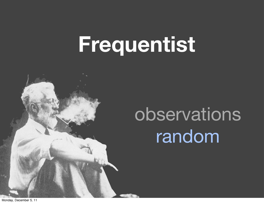
10. Frequentist observations random Monday, December 5, 11
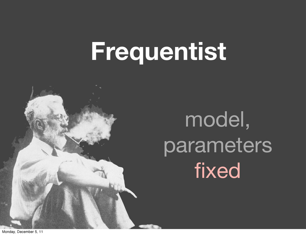
11. Frequentist model, parameters fixed Monday, December 5, 11
12. Frequentist Inference Monday, December 5, 11
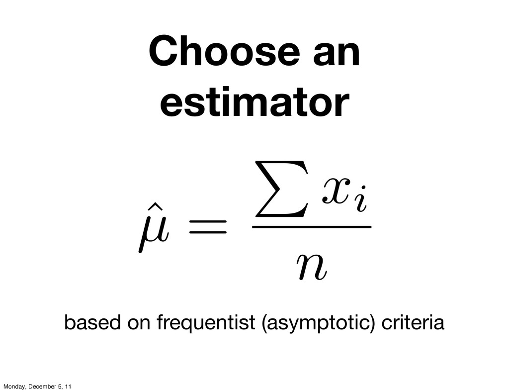
13. Choose an estimator ˆ µ = P xi n based on frequentist (asymptotic) criteria Monday, December 5, 11
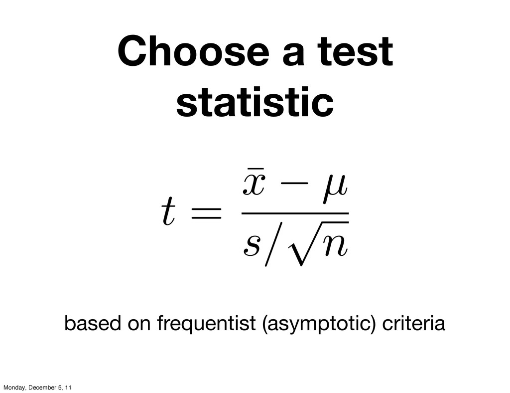
14. Choose a test statistic based on frequentist (asymptotic) criteria t = ¯ x µ s/ p n Monday, December 5, 11
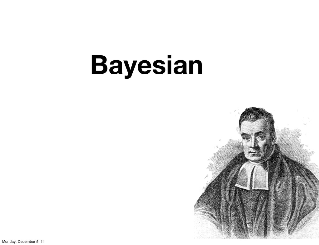
15. Bayesian Monday, December 5, 11
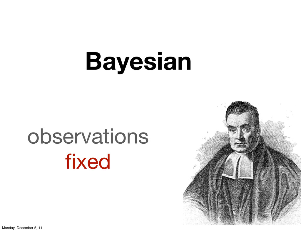
16. Bayesian observations fixed Monday, December 5, 11
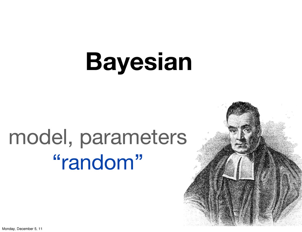
17. Bayesian model, parameters “random” Monday, December 5, 11
18. Components of Bayesian Statistics Monday, December 5, 11
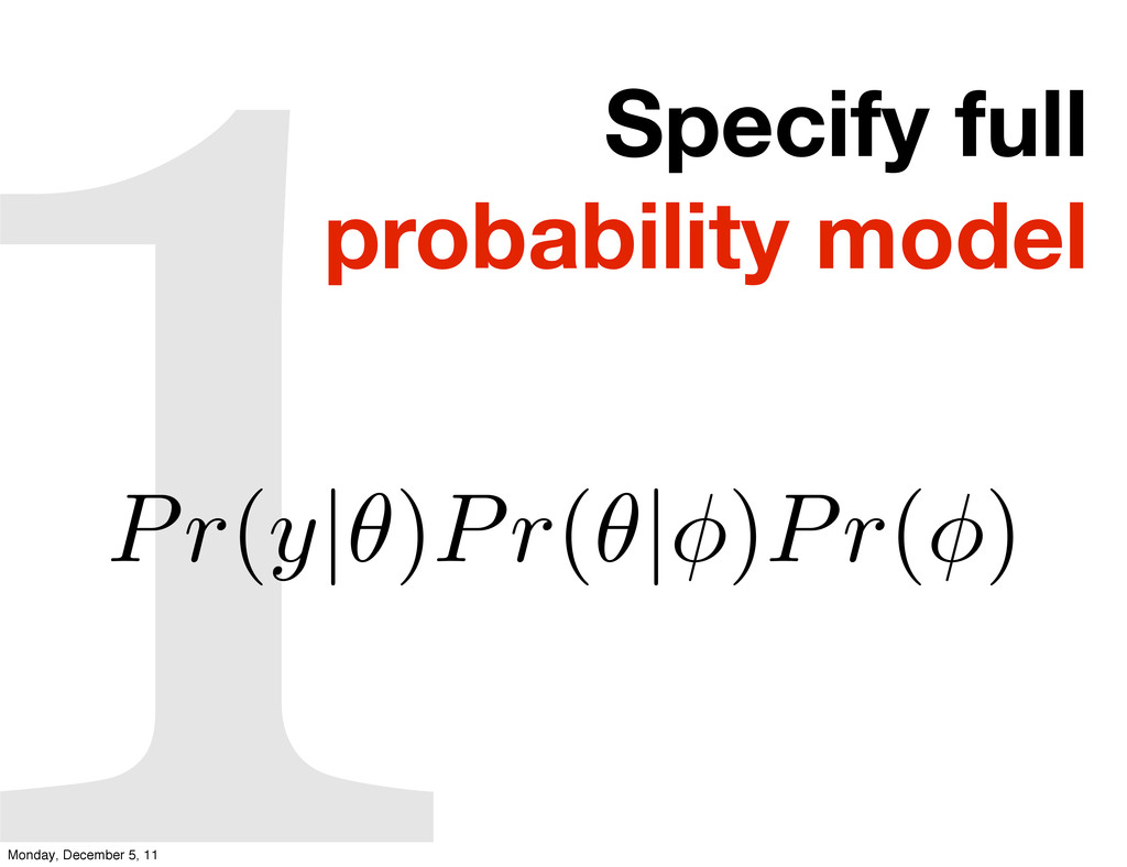
19. Specify full probability model 1 Pr(y| )Pr( |⇥)Pr(⇥) Monday, December 5, 11
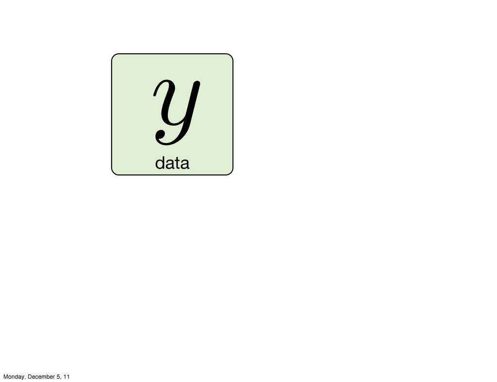
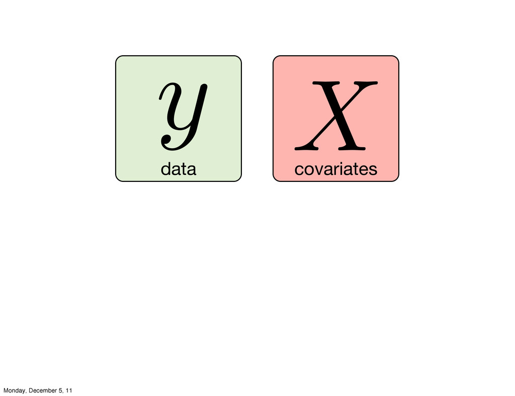
20. data y Monday, December 5, 11
21. data y covariates X Monday, December 5, 11
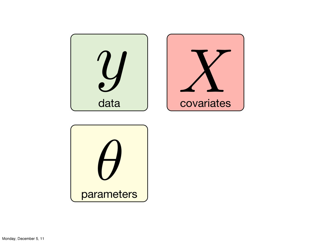
22. data y covariates X parameters ✓ Monday, December 5, 11
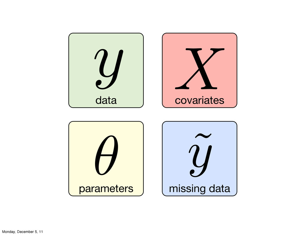
23. data y covariates X parameters ✓ missing data ˜ y Monday, December 5, 11
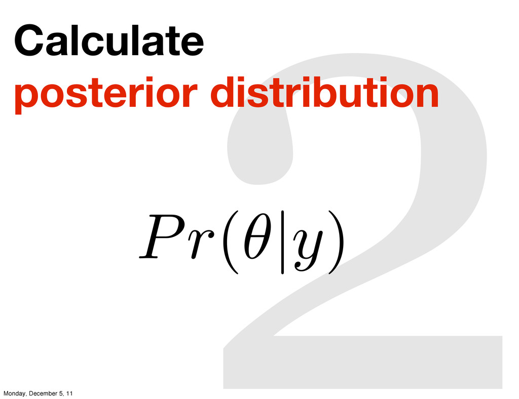
24. 2 Calculate posterior distribution Pr( |y) Monday, December 5, 11
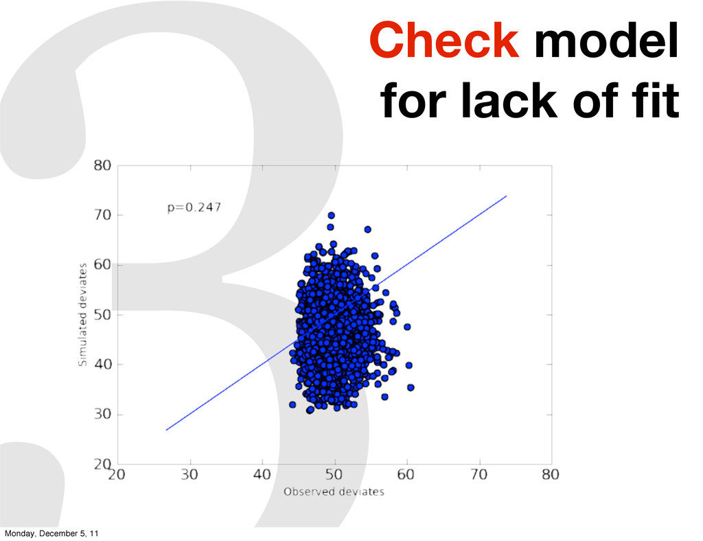
25. 3Check model for lack of fit Monday, December 5, 11
26. Why Bayes? ? Monday, December 5, 11
27. “... the Bayesian approach is attractive because it is useful. Its usefulness derives in large measure from its simplicity. Its simplicity allows the investigation of far more complex models than can be handled by the tools in the classical toolbox.” Link and Barker (2010) Monday, December 5, 11
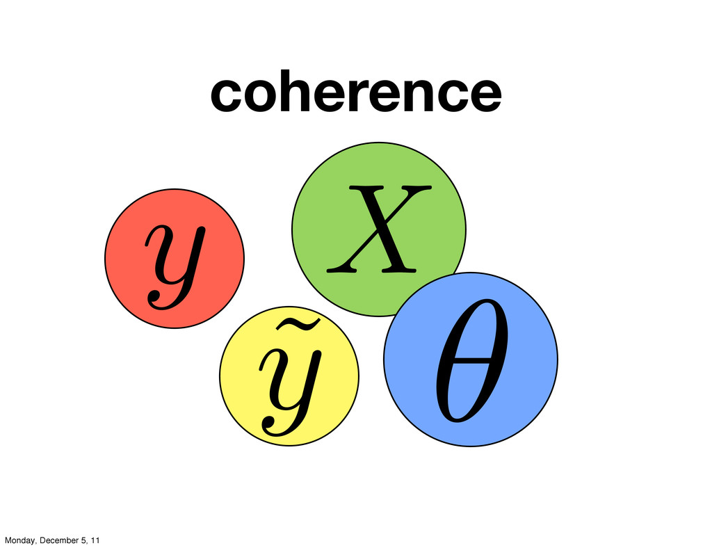
28. coherence X ˜ y y ✓ Monday, December 5, 11
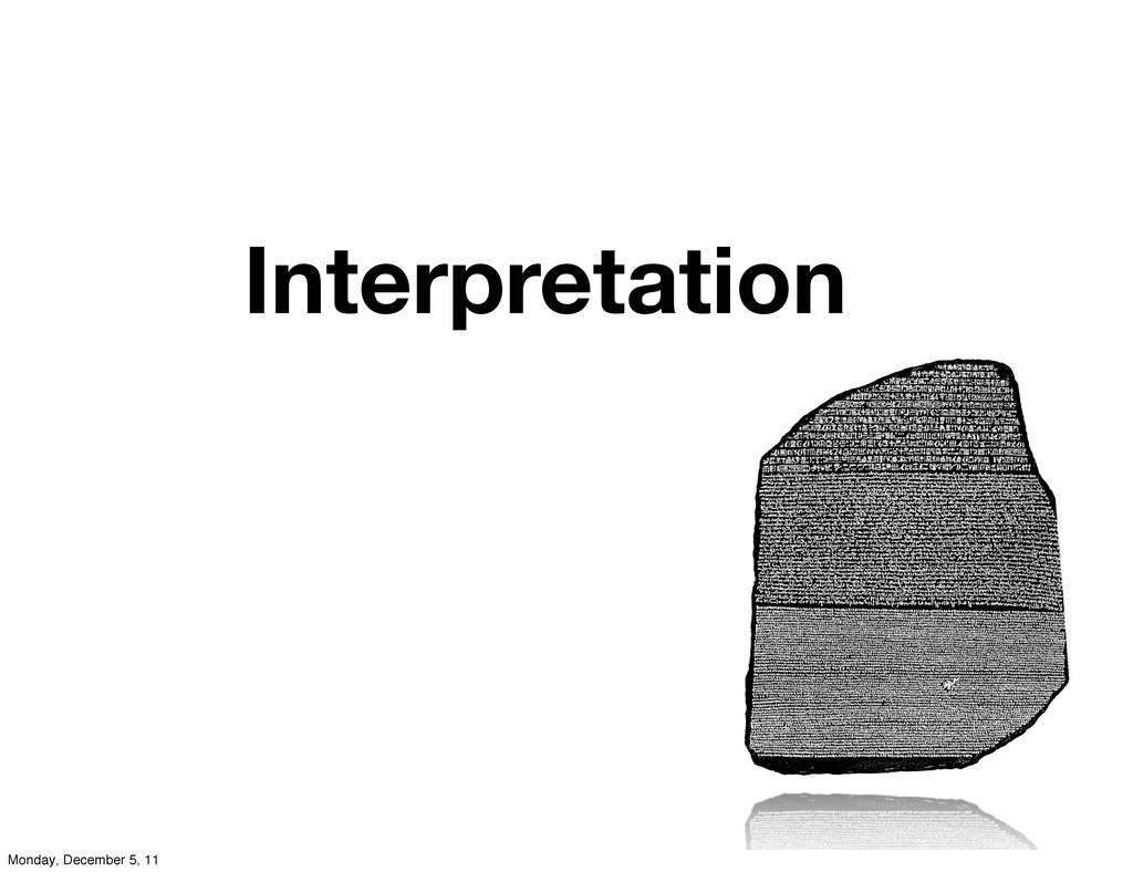
29. Interpretation Monday, December 5, 11
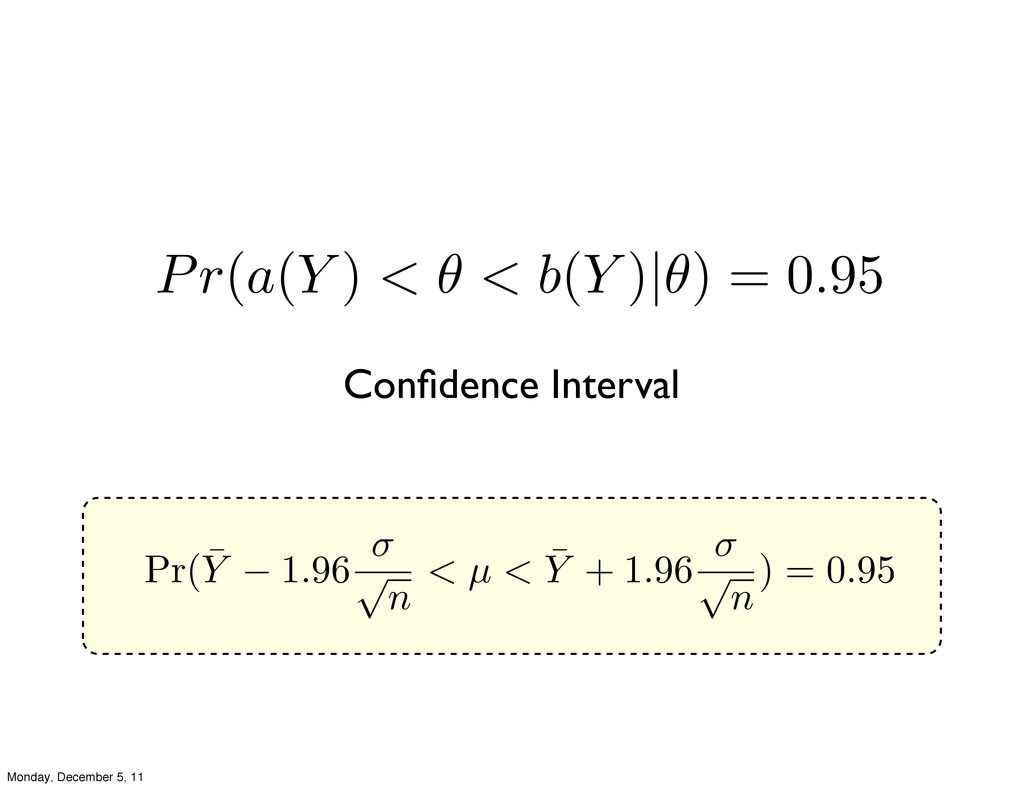
30. Pr( ¯ Y 1.96 ⇥ ⇥ n < µ < ¯ Y + 1.96 ⇥ ⇥ n ) = 0.95 Confidence Interval Pr(a(Y ) < ✓ < b(Y )|✓) = 0.95 Monday, December 5, 11
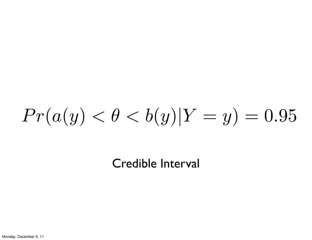
31. Credible Interval Pr(a(y) < ✓ < b(y)|Y = y) = 0.95 Monday, December 5, 11
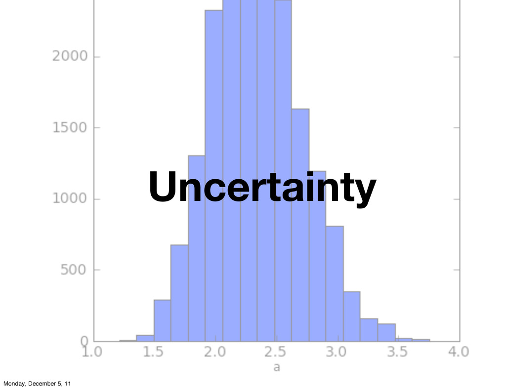
32. Uncertainty Monday, December 5, 11
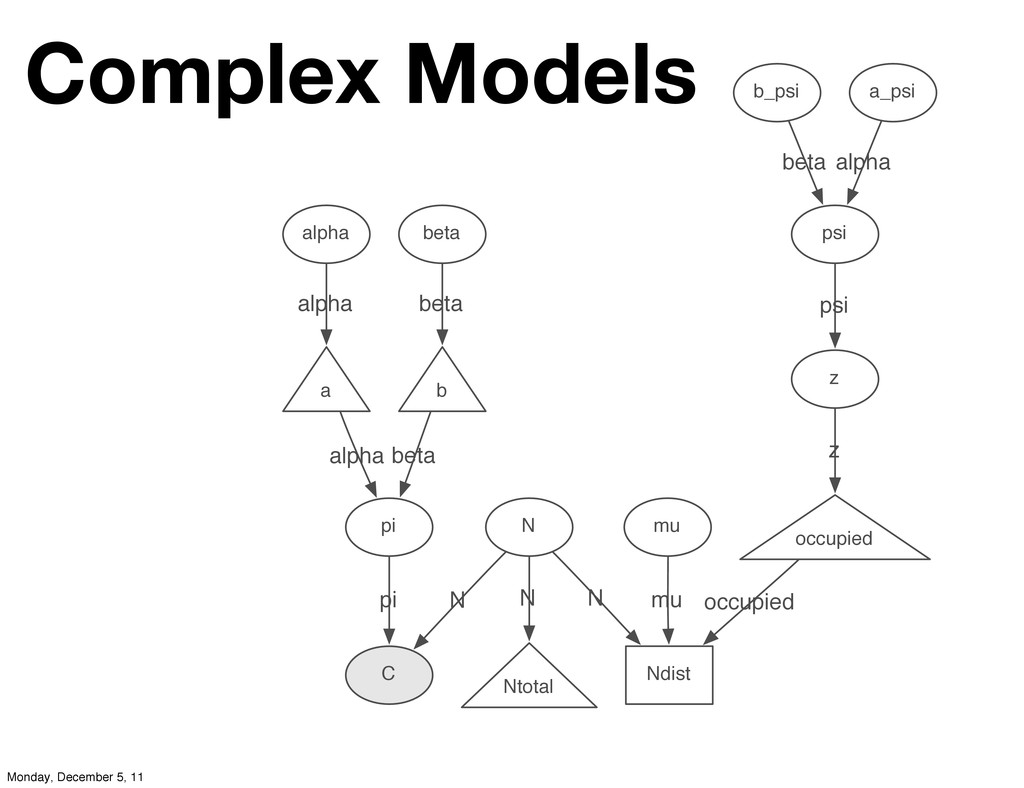
33. C alpha N z b_psi beta a_psi pi mu psi Ntotal occupied a b Ndist psi z alpha pi N beta mu occupied N alpha beta N alpha beta Complex Models Monday, December 5, 11
34. Probability Monday, December 5, 11
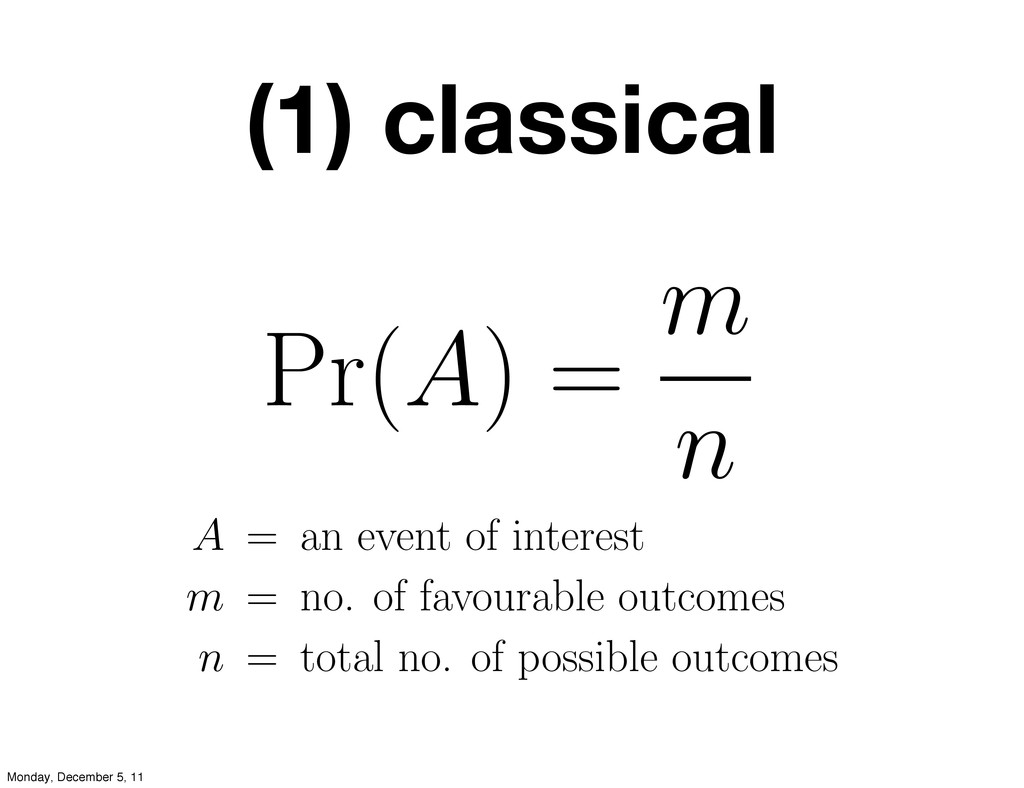
35. Pr(A) = m n A = an event of interest m = no. of favourable outcomes n = total no. of possible outcomes (1) classical Monday, December 5, 11
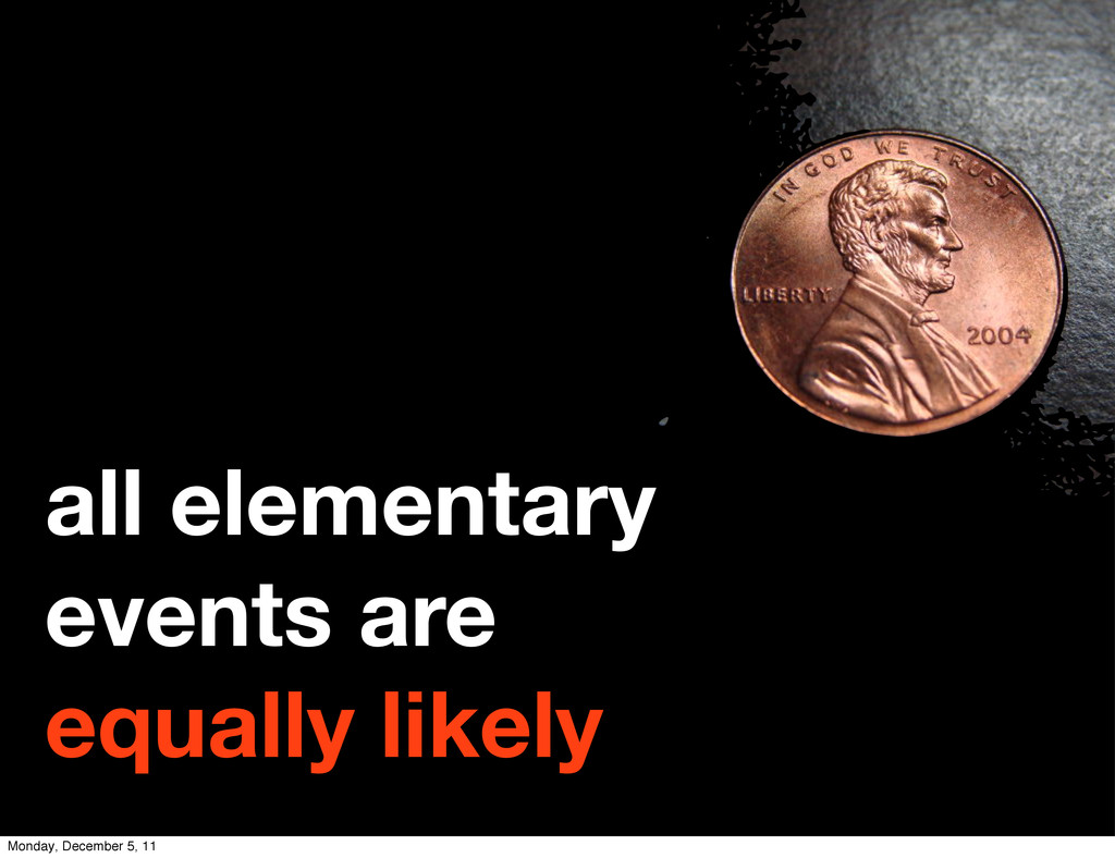
36. all elementary events are equally likely Monday, December 5, 11
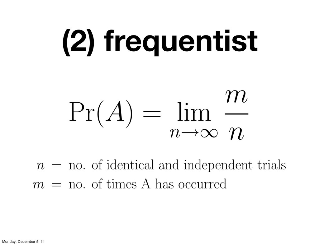
37. Pr(A) = lim n→∞ m n n = no. of identical and independent trials m = no. of times A has occurred (2) frequentist Monday, December 5, 11
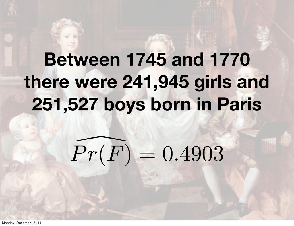
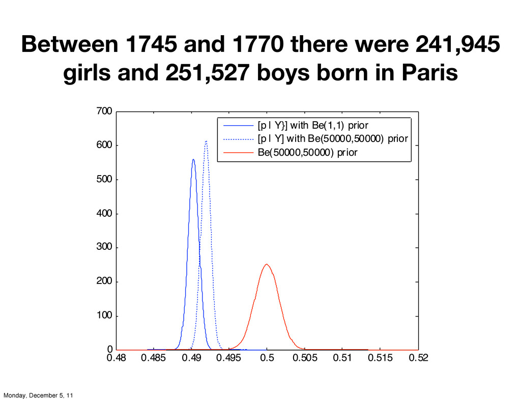
38. Between 1745 and 1770 there were 241,945 girls and 251,527 boys born in Paris Monday, December 5, 11
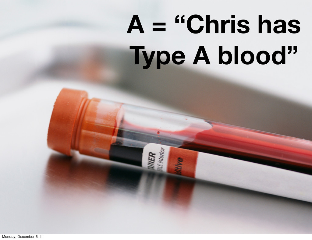
39. A = “Chris has Type A blood” Monday, December 5, 11
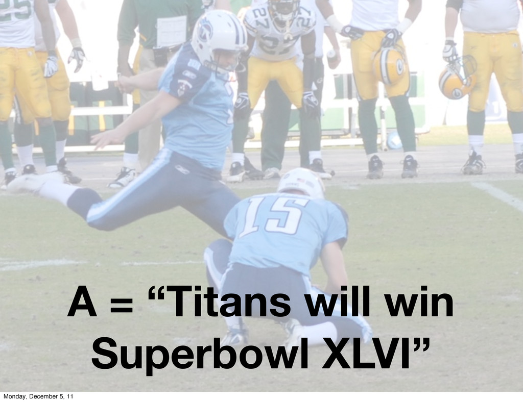
40. A = “Titans will win Superbowl XLVI” Monday, December 5, 11
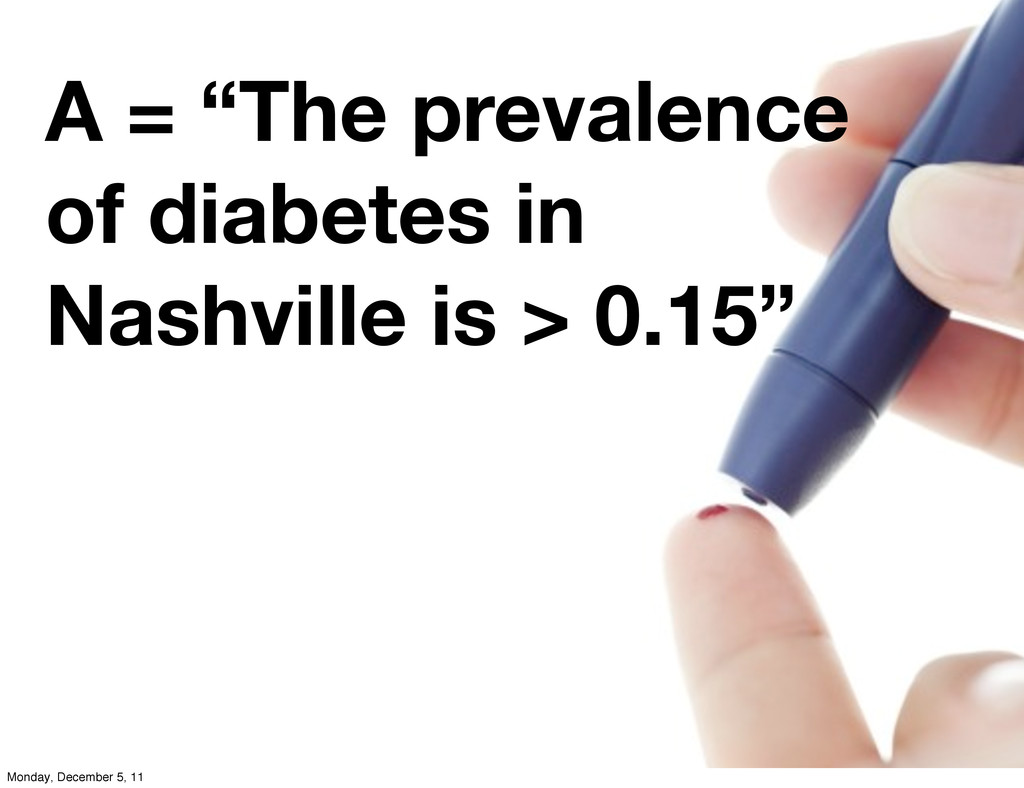
41. A = “The prevalence of diabetes in Nashville is > 0.15” Monday, December 5, 11
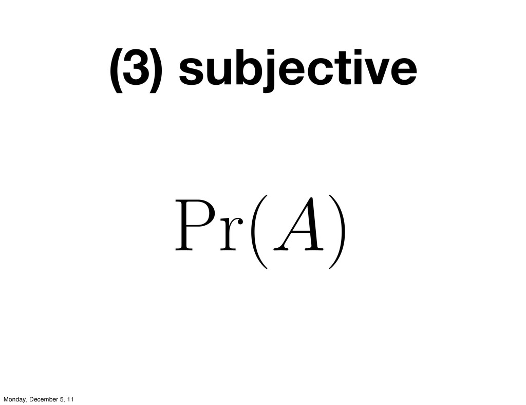
42. (3) subjective Pr(A) Monday, December 5, 11
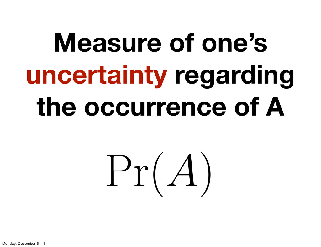
43. Measure of one’s uncertainty regarding the occurrence of A Pr(A) Monday, December 5, 11
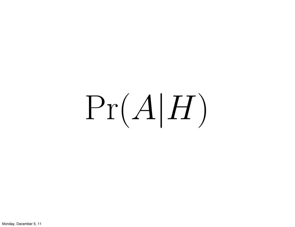
44. Pr(A|H) Monday, December 5, 11
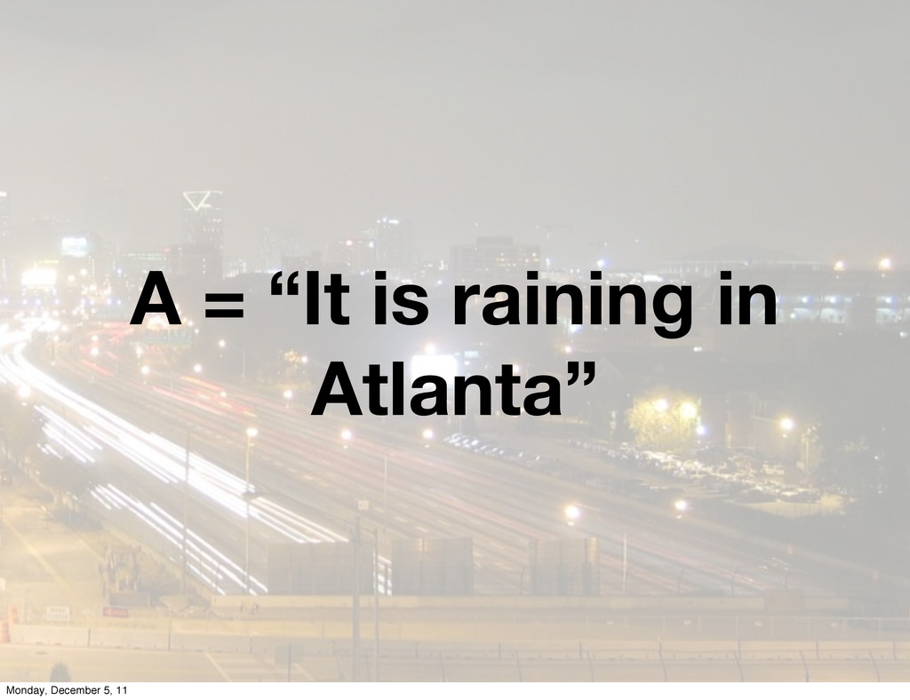
45. A = “It is raining in Atlanta” Monday, December 5, 11
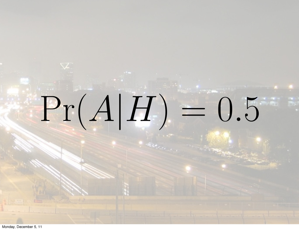
46. Pr(A|H) = 0.5 Monday, December 5, 11
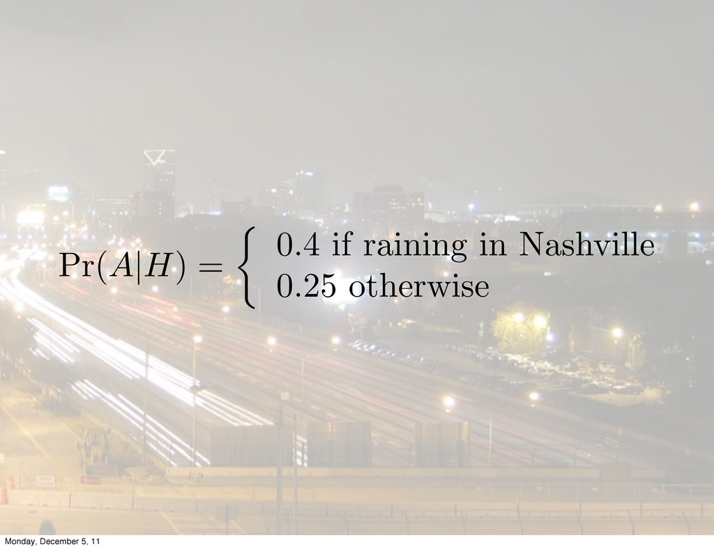
47. Pr( A|H ) = ⇢ 0 . 4 if raining in Nashville 0 . 25 otherwise Monday, December 5, 11
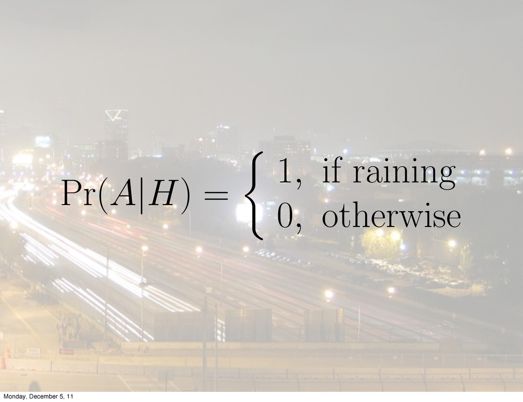
48. Pr(A|H) = 1, if raining 0, otherwise Monday, December 5, 11
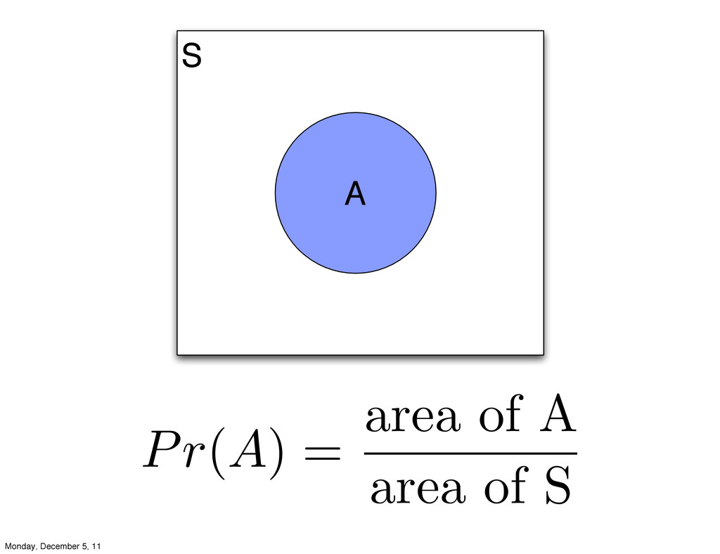
49. S A Pr(A) = area of A area of S Monday, December 5, 11
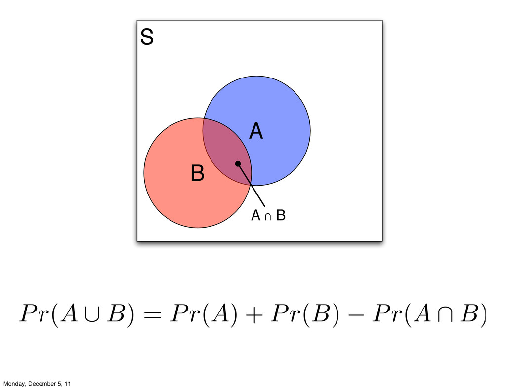
50. S A B A ∩ B Pr(A ⇥ B) = Pr(A) + Pr(B) Pr(A ⇤ B) Monday, December 5, 11
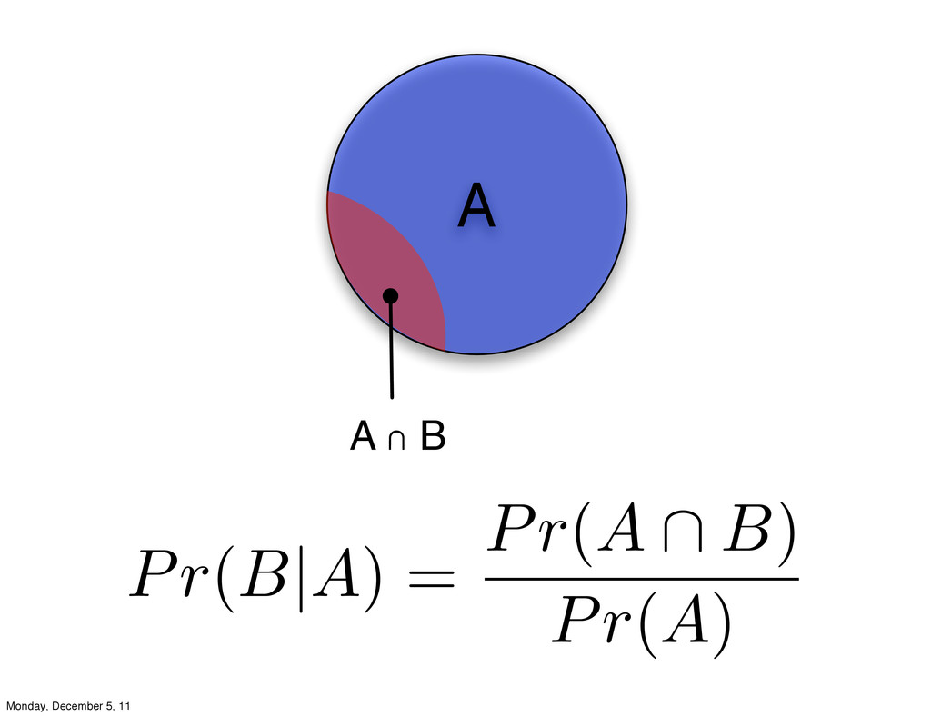
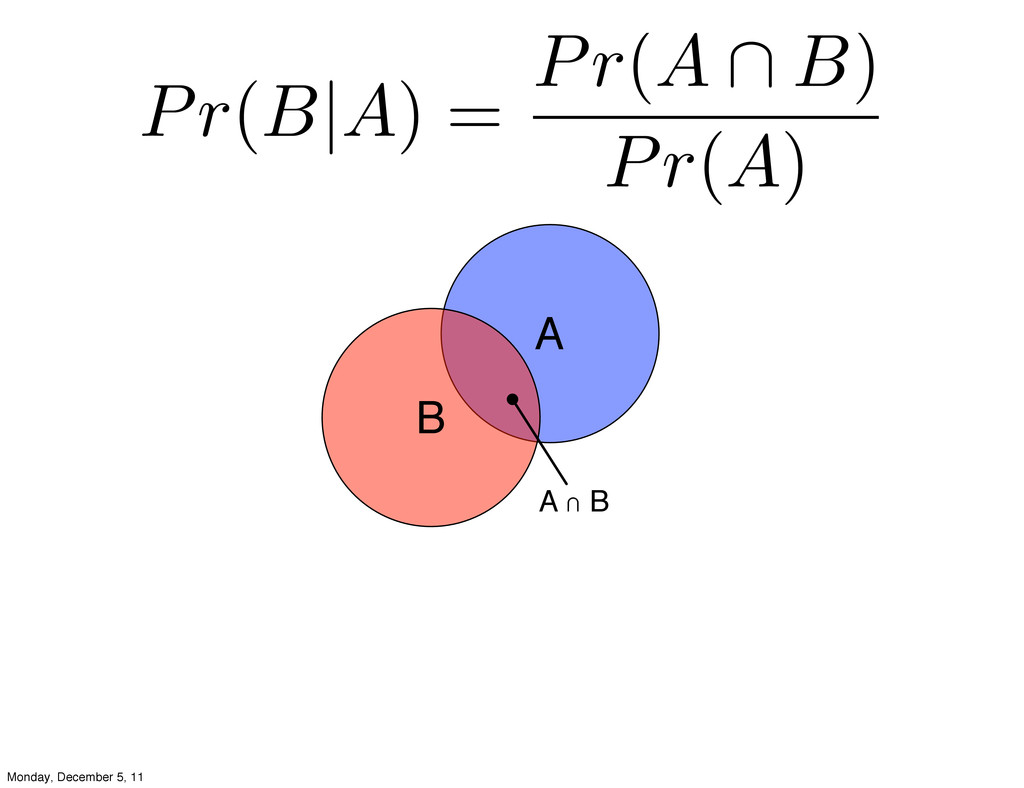
51. A A ∩ B Pr(B|A) = Pr(A B) Pr(A) Monday, December 5, 11
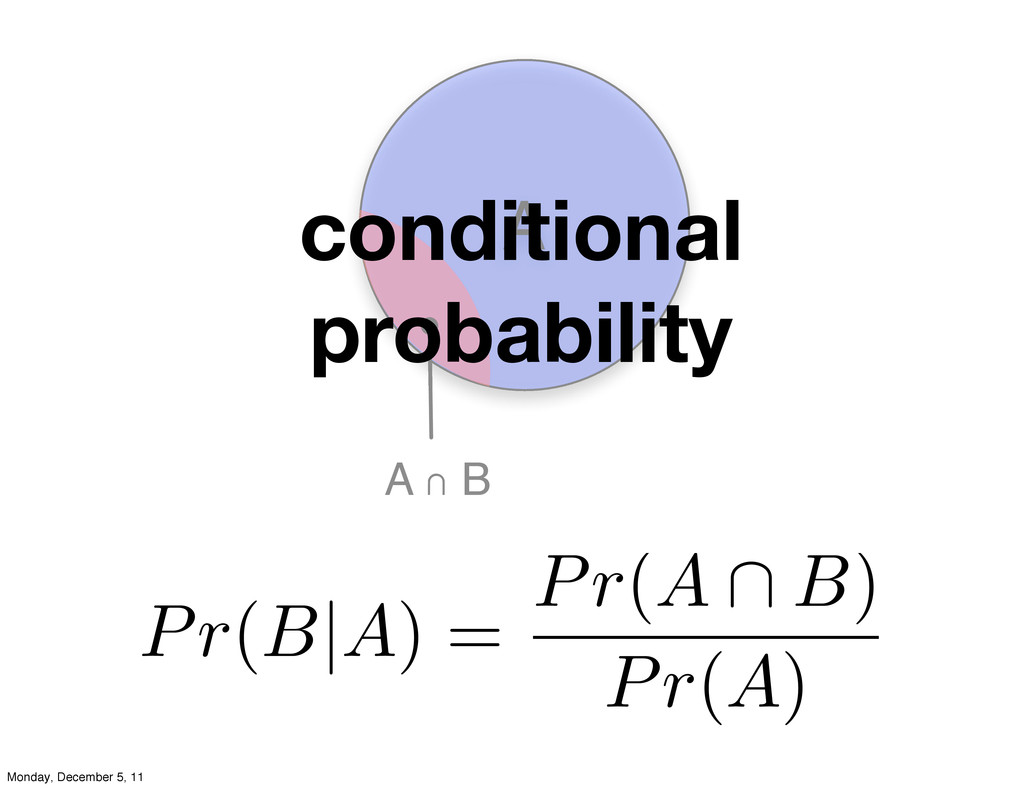
52. A A ∩ B conditional probability Pr(B|A) = Pr(A B) Pr(A) Monday, December 5, 11
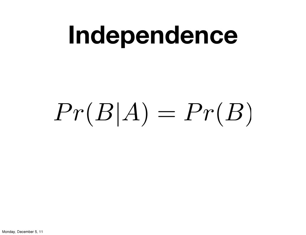
53. Independence Pr(B|A) = Pr(B) Monday, December 5, 11
54. S A B A ∩ B Pr(B|A) = Pr(A B) Pr(A) Monday, December 5, 11
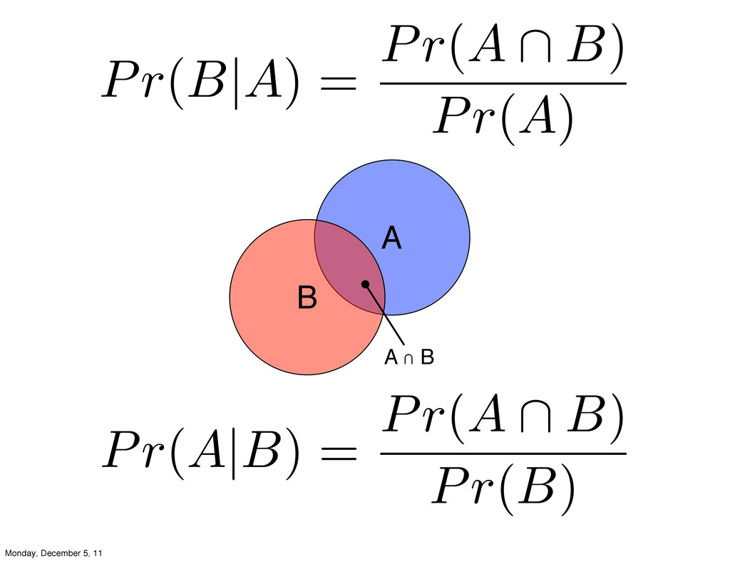
55. S A B A ∩ B Pr(A|B) = Pr(A B) Pr(B) Pr(B|A) = Pr(A B) Pr(A) Monday, December 5, 11
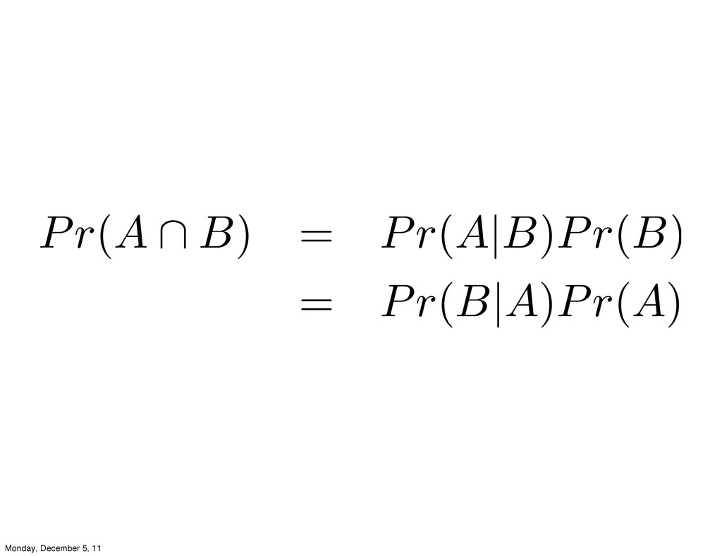
56. Pr(A B) = Pr(A|B)Pr(B) = Pr(B|A)Pr(A) Monday, December 5, 11
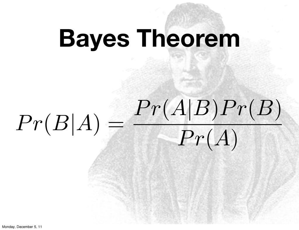
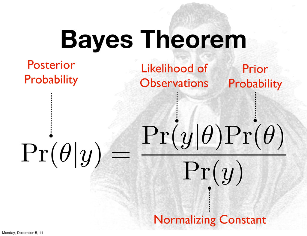
57. Bayes Theorem Pr(B|A) = Pr(A|B)Pr(B) Pr(A) Monday, December 5, 11
58. Bayes Theorem Pr( |y) = Pr(y| )Pr( ) Pr(y) Posterior Probability Prior Probability Likelihood of Observations Normalizing Constant Monday, December 5, 11
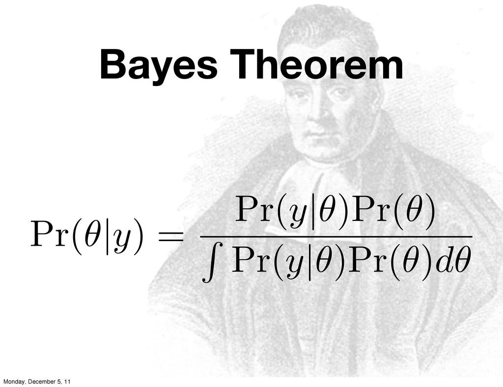
59. Bayes Theorem Pr( |y) = Pr(y| )Pr( ) R Pr(y| )Pr( )d Monday, December 5, 11
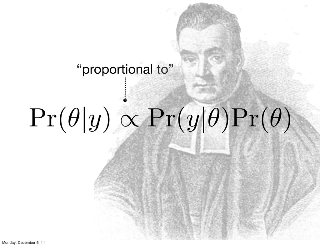
60. “proportional to” Pr( |y) Pr(y| )Pr( ) Monday, December 5, 11
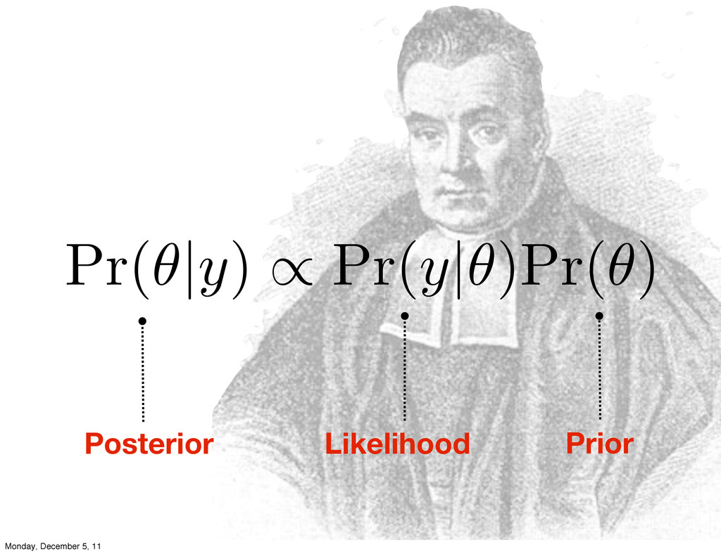
61. Pr( |y) Pr(y| )Pr( ) Posterior Prior Likelihood Monday, December 5, 11
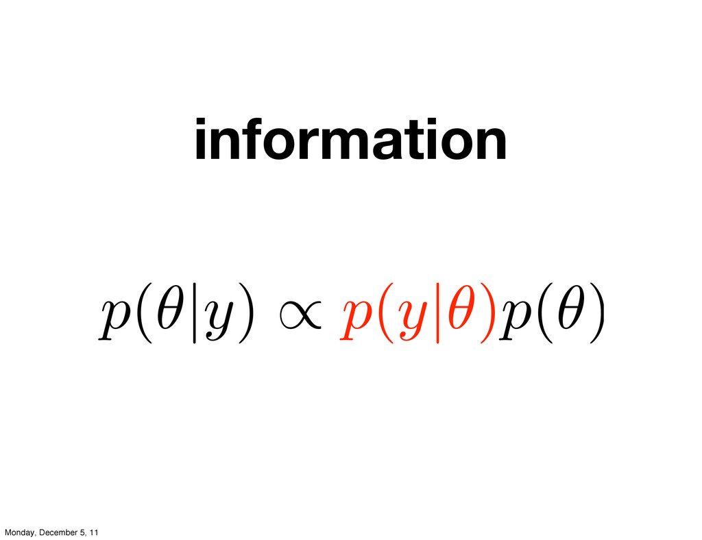
62. information p( |y) p(y| )p( ) Monday, December 5, 11
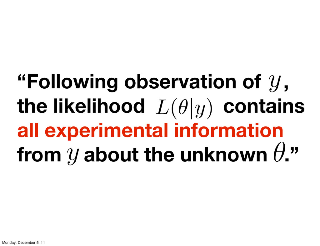
63. “Following observation of , the likelihood contains all experimental information from about the unknown .” θ y y L(✓|y) Monday, December 5, 11
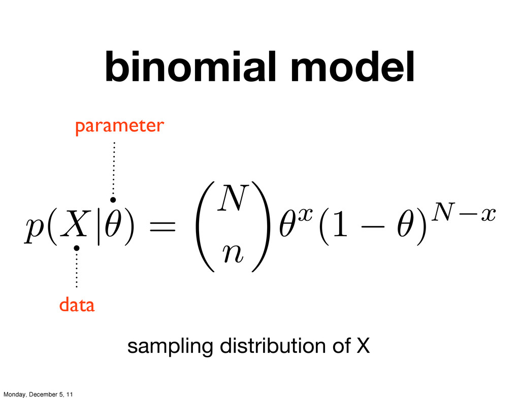
64. binomial model data parameter sampling distribution of X p(X|✓) = ✓ N n ◆ ✓x (1 ✓)N x Monday, December 5, 11
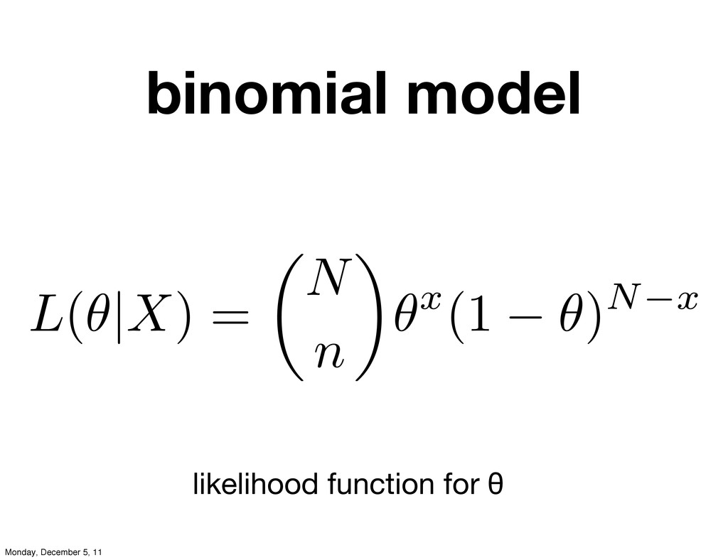
65. binomial model likelihood function for θ L(✓|X) = ✓ N n ◆ ✓x (1 ✓)N x Monday, December 5, 11
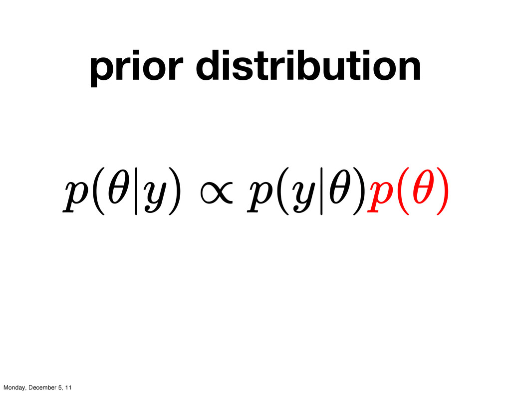
66. prior distribution p(θ|y) ∝ p(y|θ)p(θ) Monday, December 5, 11
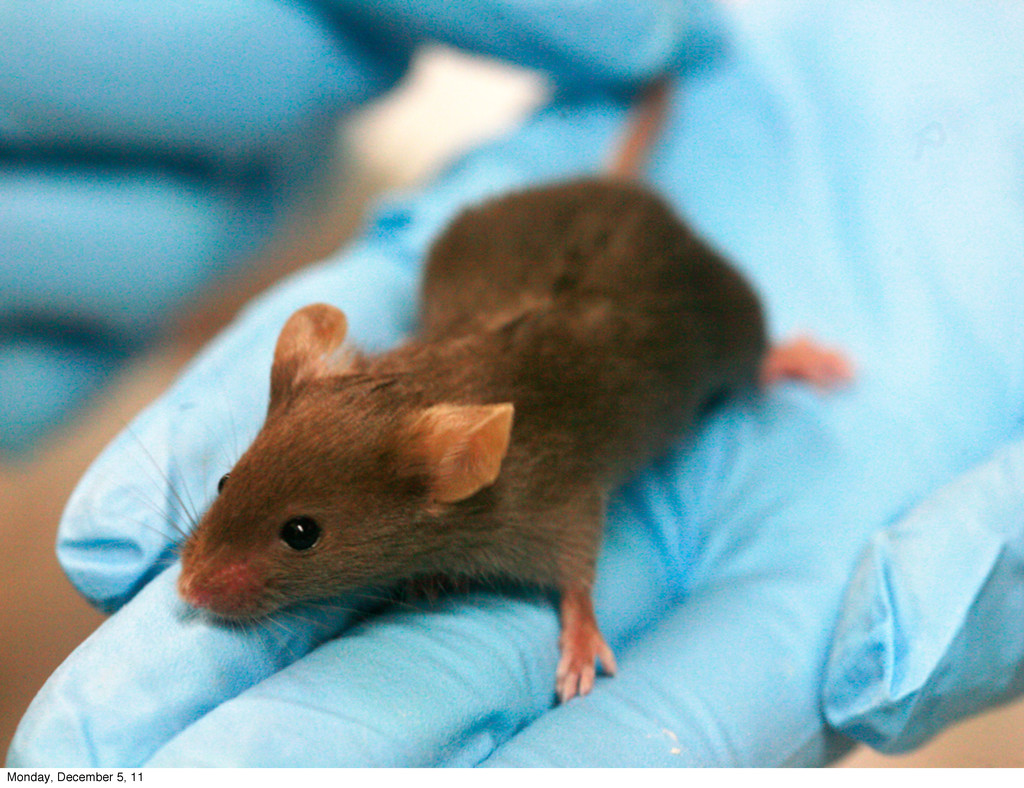
67. Prior as population distribution Monday, December 5, 11
68. Monday, December 5, 11
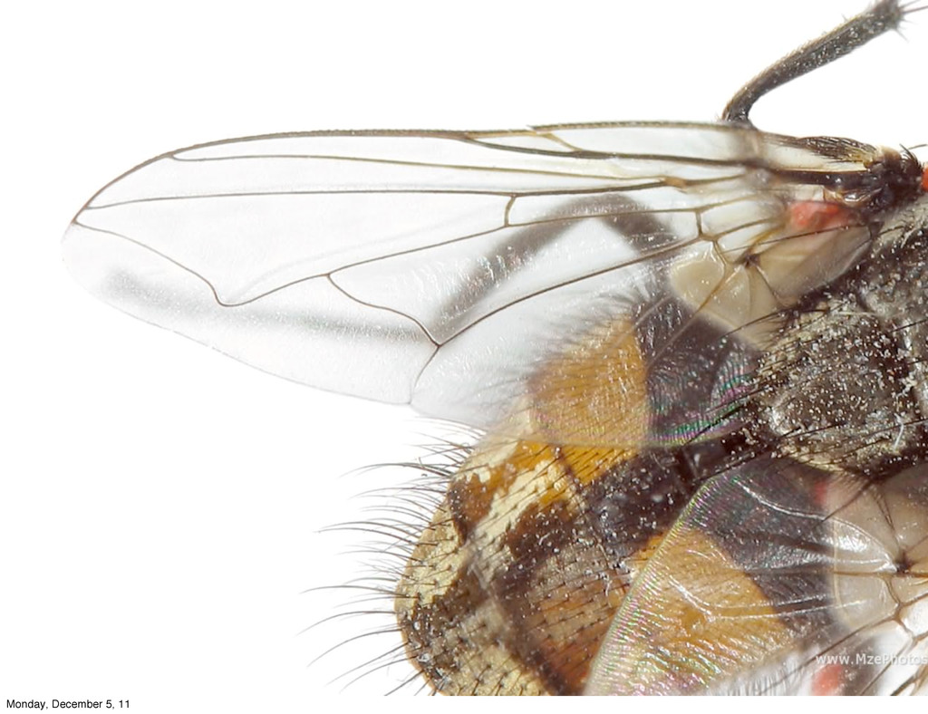
69. Prior as information state Monday, December 5, 11
70. Monday, December 5, 11
71. All plausible values Monday, December 5, 11
72. Between 1745 and 1770 there were 241,945 girls and 251,527 boys born in Paris Monday, December 5, 11
73. Bayesian analysis is subjective Monday, December 5, 11
74. Statistical analysis is subjective Monday, December 5, 11
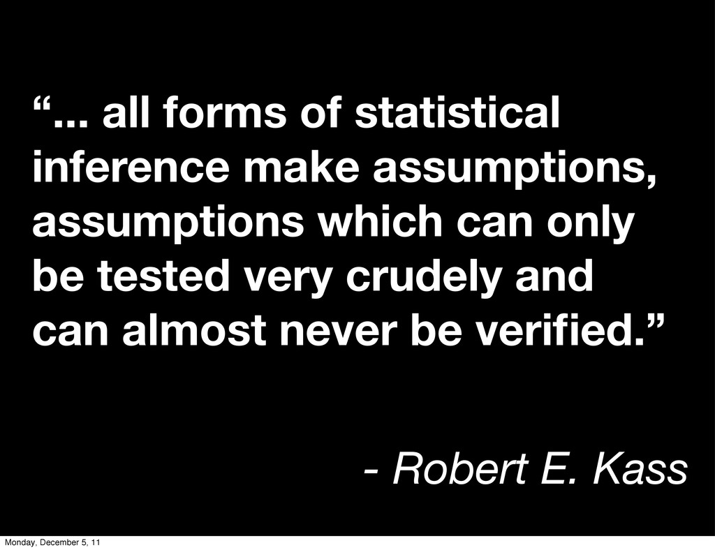
75. “... all forms of statistical inference make assumptions, assumptions which can only be tested very crudely and can almost never be verified.” - Robert E. Kass Monday, December 5, 11
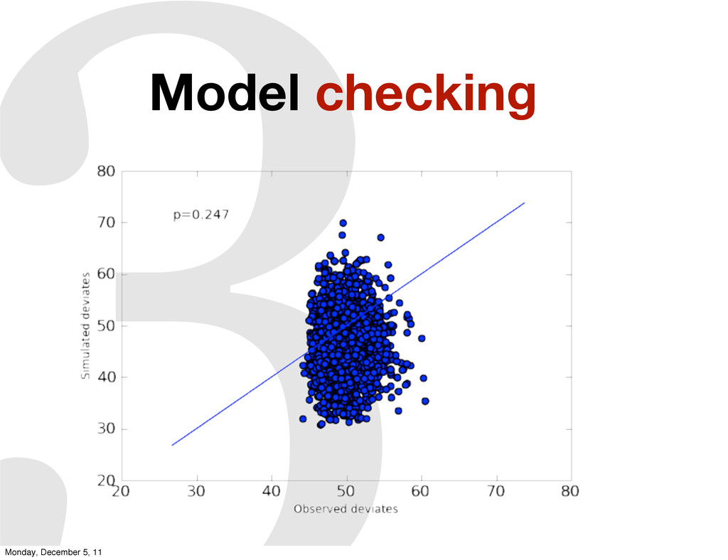
76. 3 Model checking Monday, December 5, 11
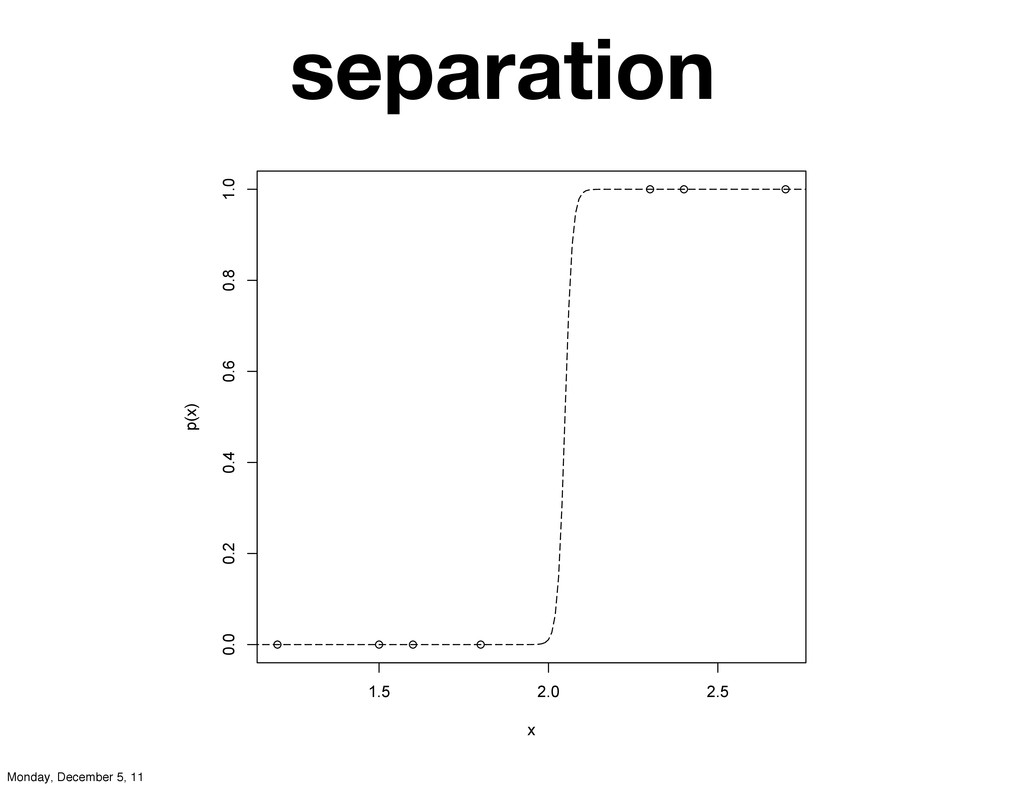
77. 1.5 2.0 2.5 0.0 0.2 0.4 0.6 0.8 1.0 x p(x) separation Monday, December 5, 11
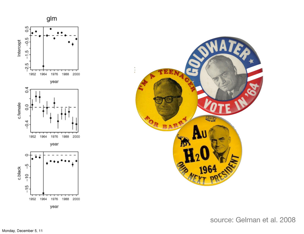
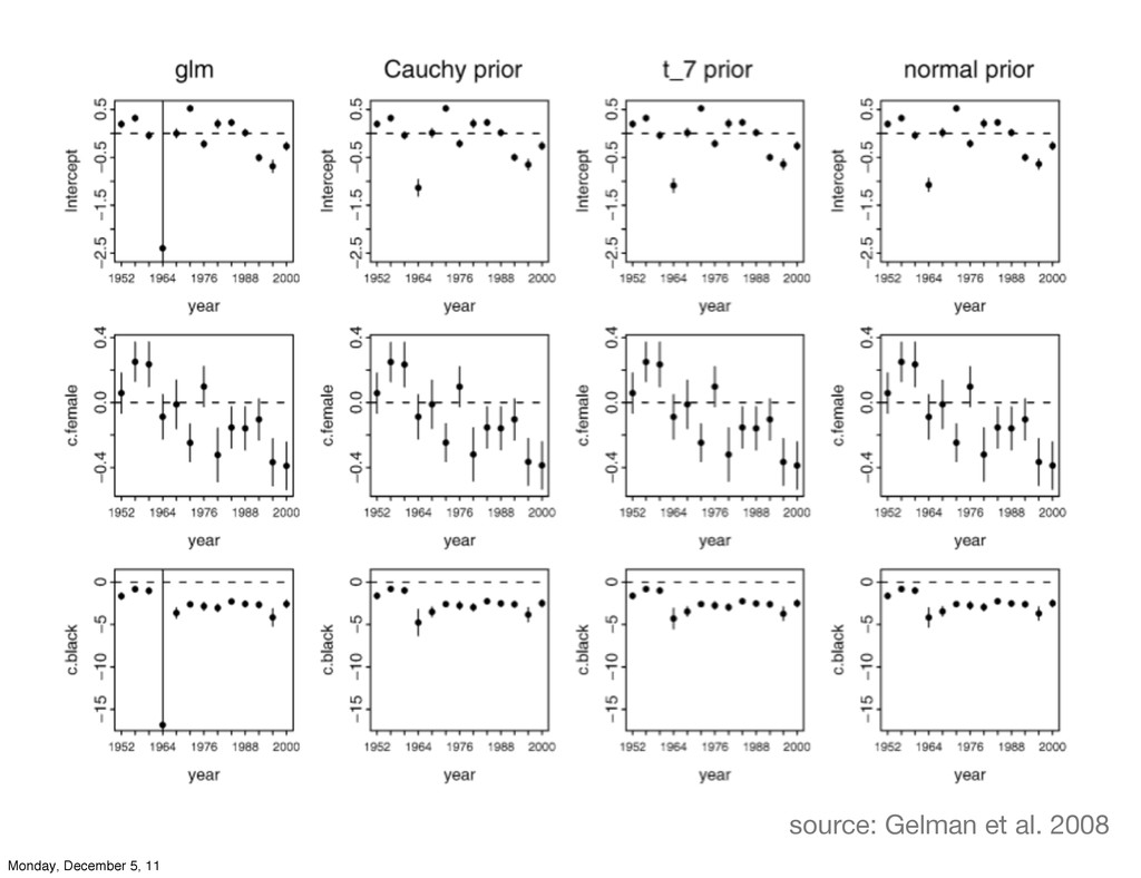
78. source: Gelman et al. 2008 Monday, December 5, 11
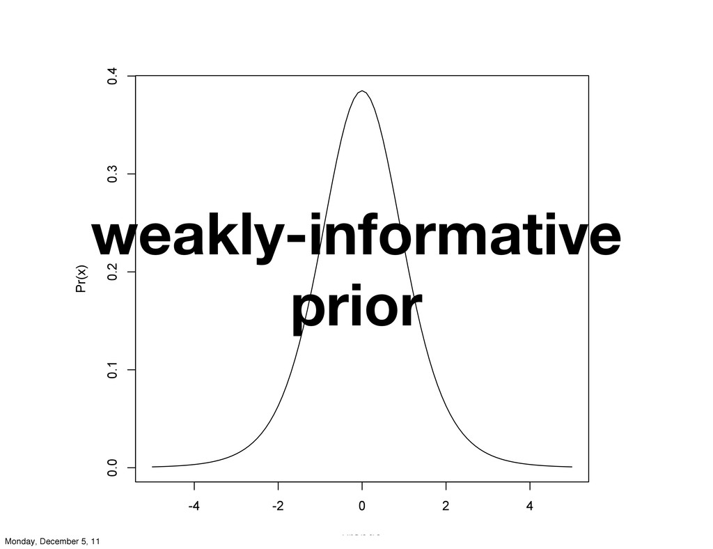
79. weakly-informative prior -4 -2 0 2 4 0.0 0.1 0.2 0.3 0.4 xrange Pr(x) Monday, December 5, 11
80. source: Gelman et al. 2008 Monday, December 5, 11
81. example: genetic probabilities Monday, December 5, 11
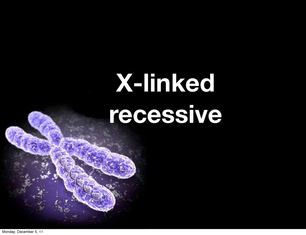
82. X-linked recessive Monday, December 5, 11
83. Monday, December 5, 11
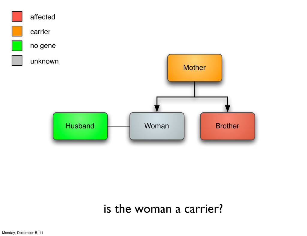
84. affected carrier no gene unknown Woman Husband Brother Mother is the woman a carrier? Monday, December 5, 11
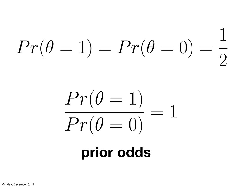
85. Pr(θ = 1) = Pr(θ = 0) = 1 2 Pr(θ = 1) Pr(θ = 0) = 1 prior odds Monday, December 5, 11
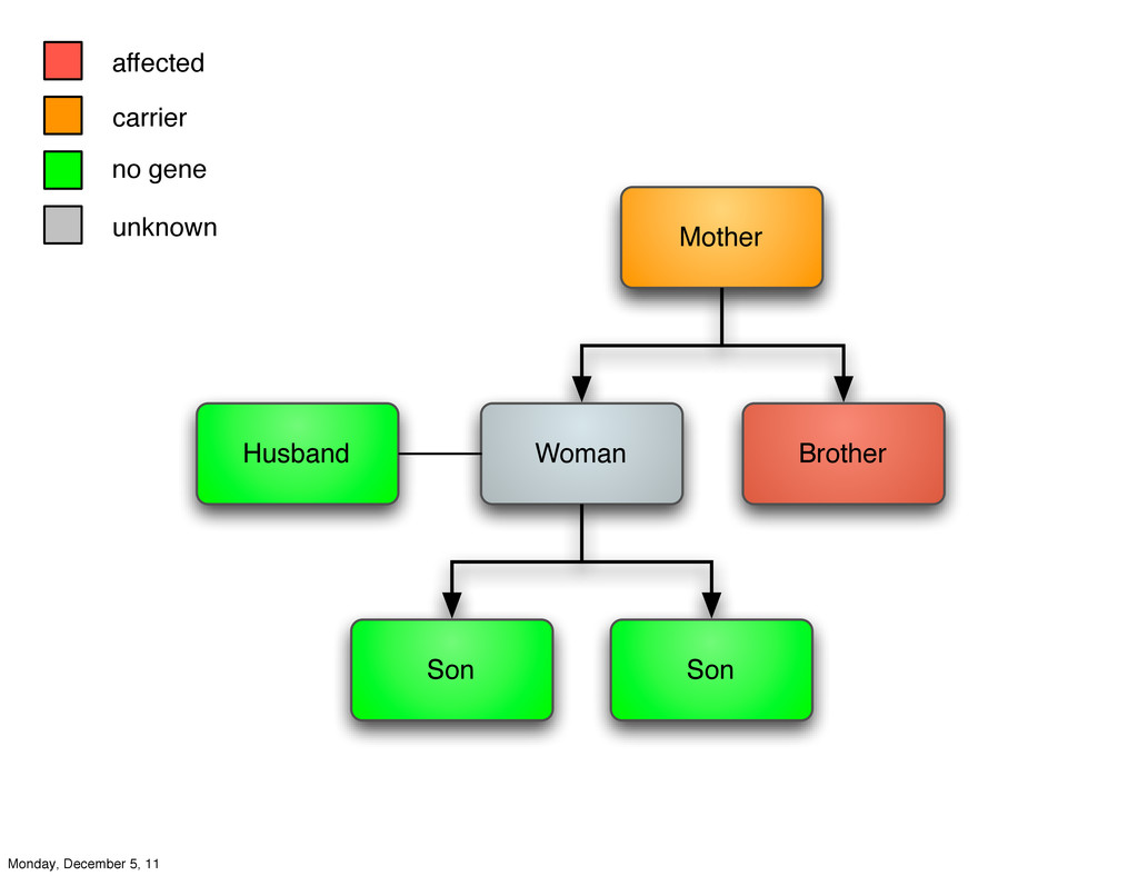
86. affected carrier no gene unknown Woman Husband Brother Son Son Mother Monday, December 5, 11
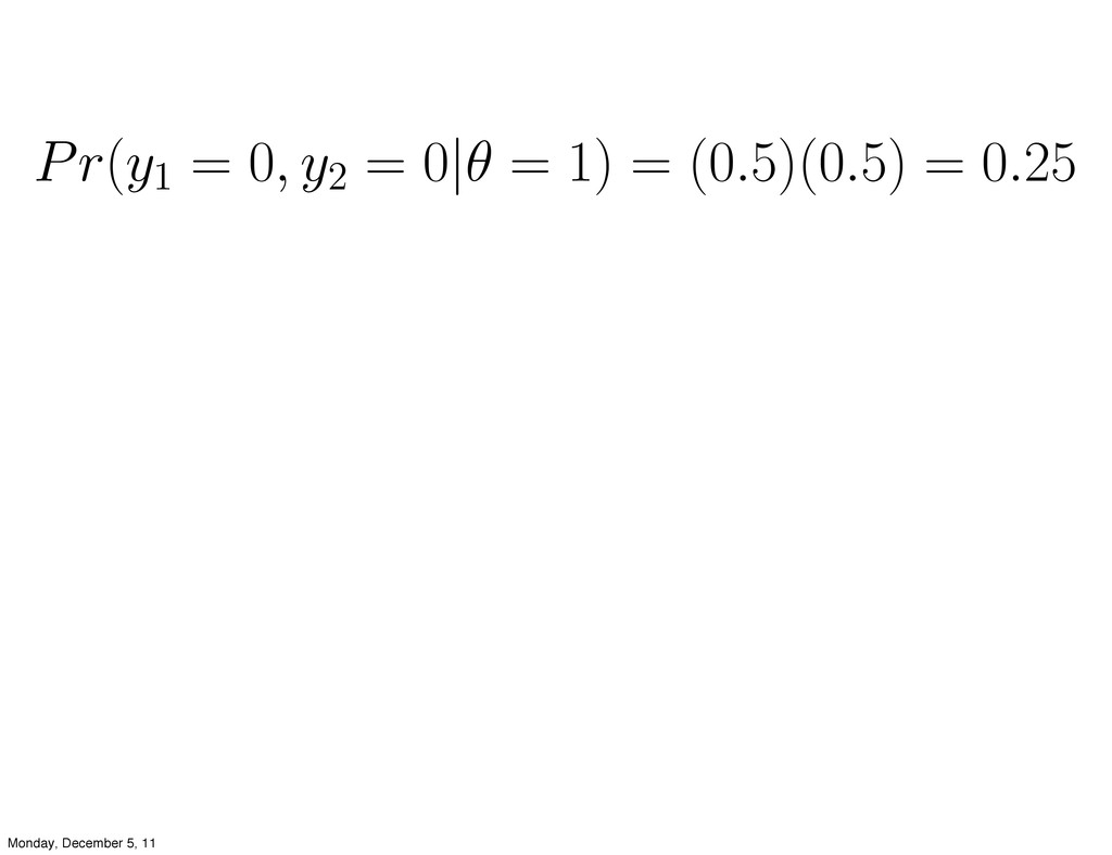
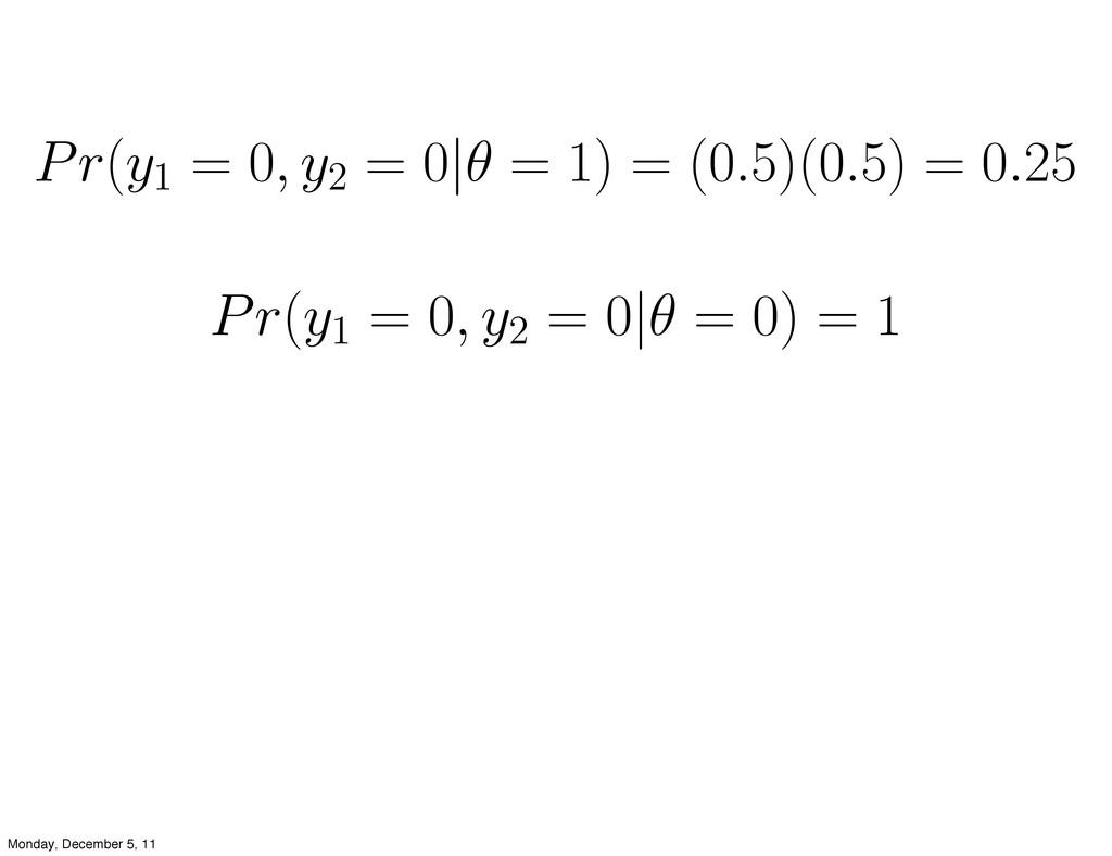
87. Pr(y1 = 0, y2 = 0|θ = 1) = (0.5)(0.5) = 0.25 Monday, December 5, 11
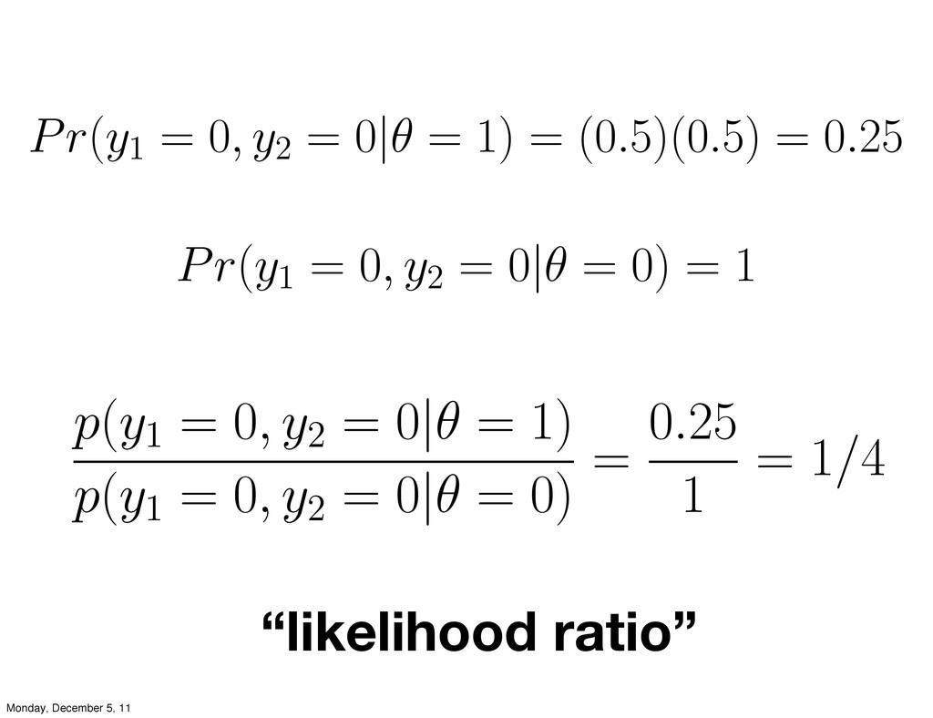
88. Pr(y1 = 0, y2 = 0|θ = 1) = (0.5)(0.5) = 0.25 Pr(y1 = 0, y2 = 0|θ = 0) = 1 Monday, December 5, 11
89. Pr(y1 = 0, y2 = 0|θ = 1) = (0.5)(0.5) = 0.25 Pr(y1 = 0, y2 = 0|θ = 0) = 1 “likelihood ratio” p(y1 = 0, y2 = 0|θ = 1) p(y1 = 0, y2 = 0|θ = 0) = 0.25 1 = 1/4 Monday, December 5, 11
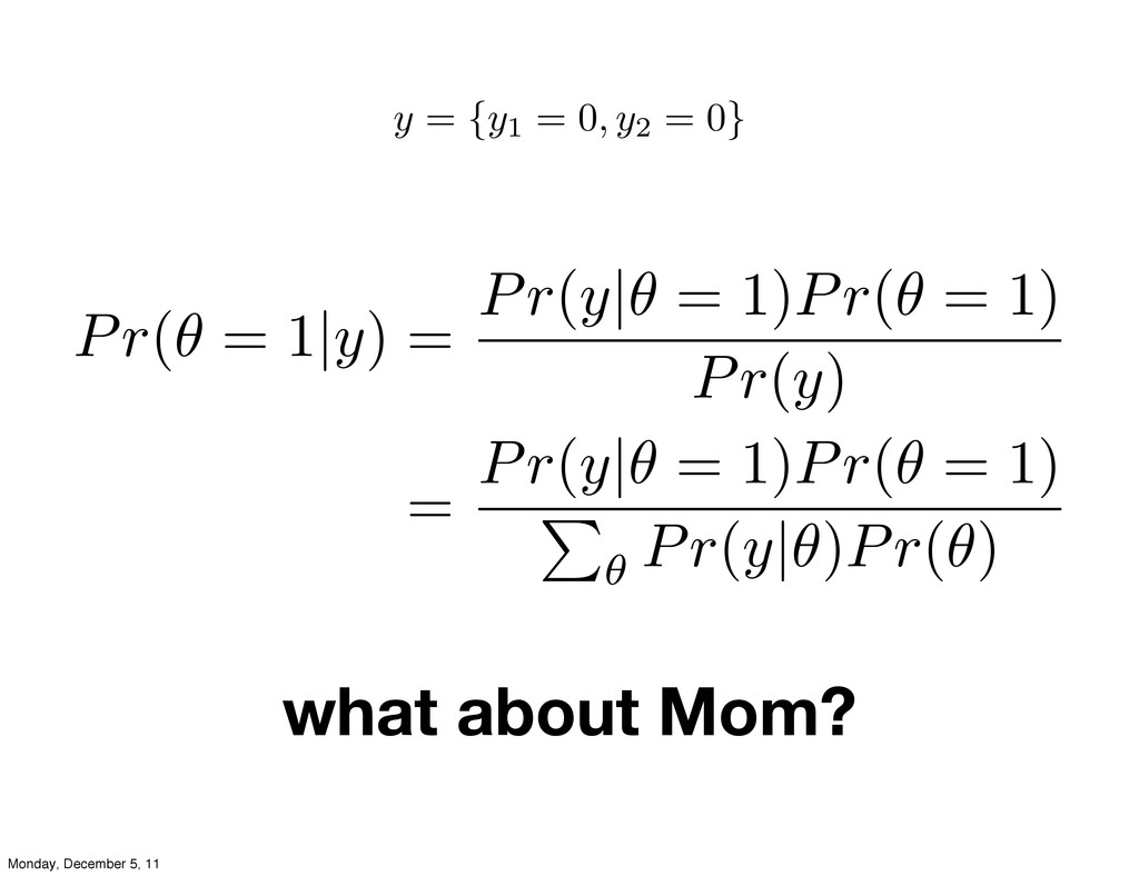
90. what about Mom? Monday, December 5, 11
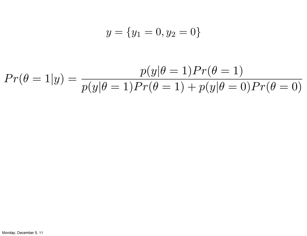
91. what about Mom? y = {y1 = 0, y2 = 0} Pr( = 1|y) = Pr(y| = 1)Pr( = 1) Pr(y) = Pr(y| = 1)Pr( = 1) P ✓ Pr(y| )Pr( ) Monday, December 5, 11
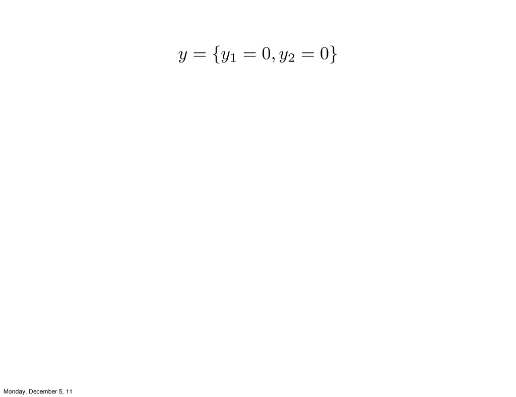
92. y = {y1 = 0, y2 = 0} Monday, December 5, 11
93. Pr( = 1|y) = p(y| = 1)Pr( = 1) p(y| = 1)Pr( = 1) + p(y| = 0)Pr( = 0) y = {y1 = 0, y2 = 0} Monday, December 5, 11
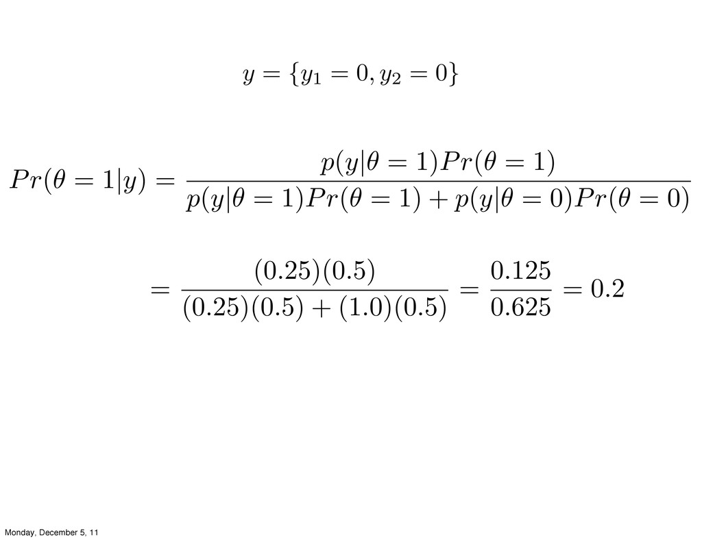
94. Pr( = 1|y) = p(y| = 1)Pr( = 1) p(y| = 1)Pr( = 1) + p(y| = 0)Pr( = 0) = (0.25)(0.5) (0.25)(0.5) + (1.0)(0.5) = 0.125 0.625 = 0.2 y = {y1 = 0, y2 = 0} Monday, December 5, 11
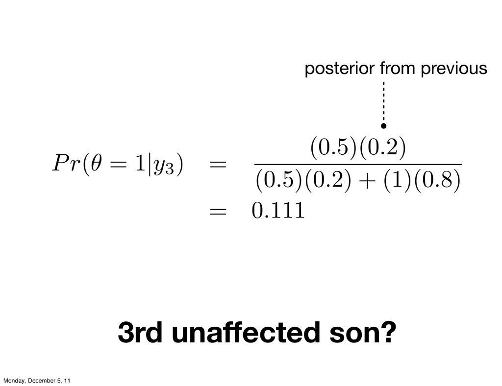
95. 3rd unaffected son? Pr( = 1|y3 ) = (0.5)(0.2) (0.5)(0.2) + (1)(0.8) = 0.111 posterior from previous Monday, December 5, 11
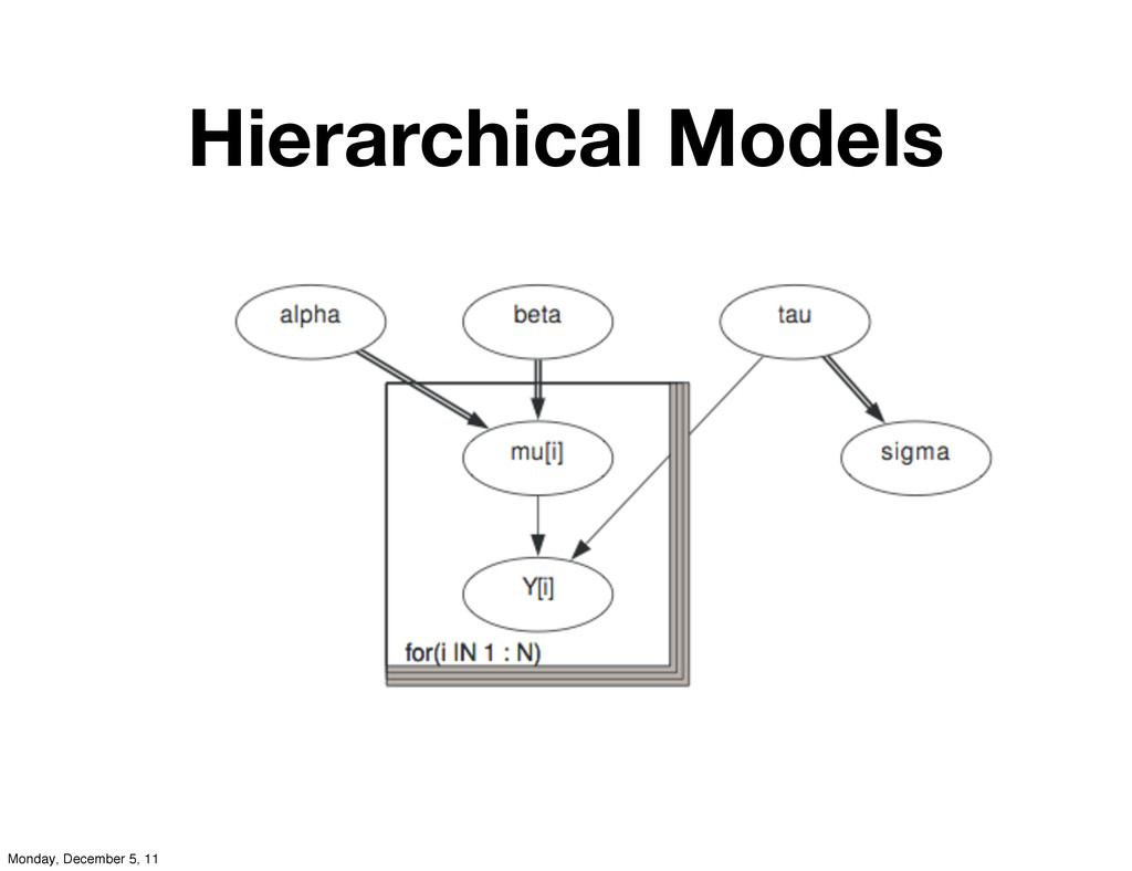
96. Hierarchical Models Monday, December 5, 11
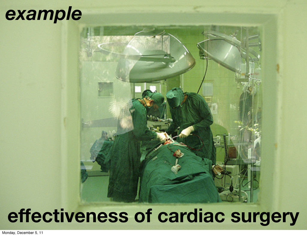
97. effectiveness of cardiac surgery example Monday, December 5, 11
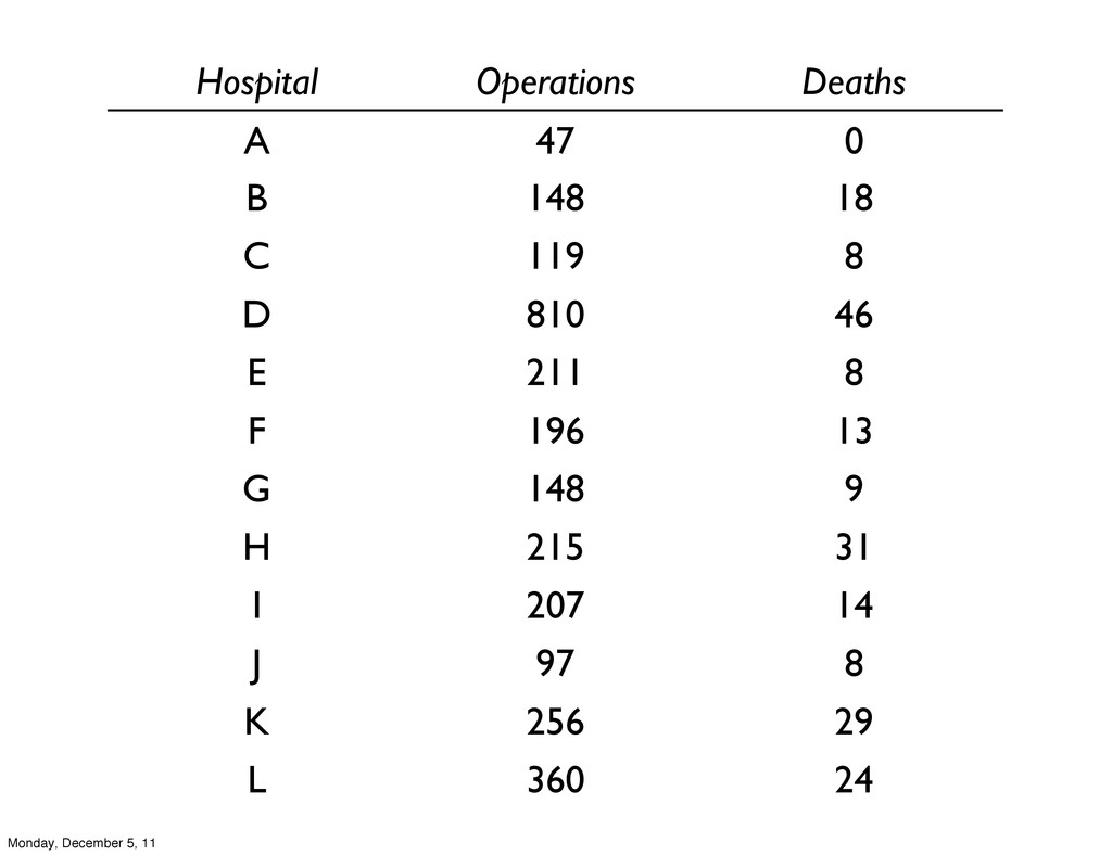
98. Hospital Operations Deaths A 47 0 B 148 18 C 119 8 D 810 46 E 211 8 F 196 13 G 148 9 H 215 31 I 207 14 J 97 8 K 256 29 L 360 24 Monday, December 5, 11
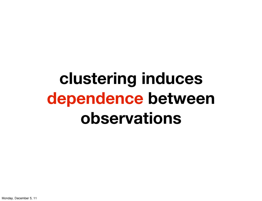
99. clustering induces dependence between observations Monday, December 5, 11
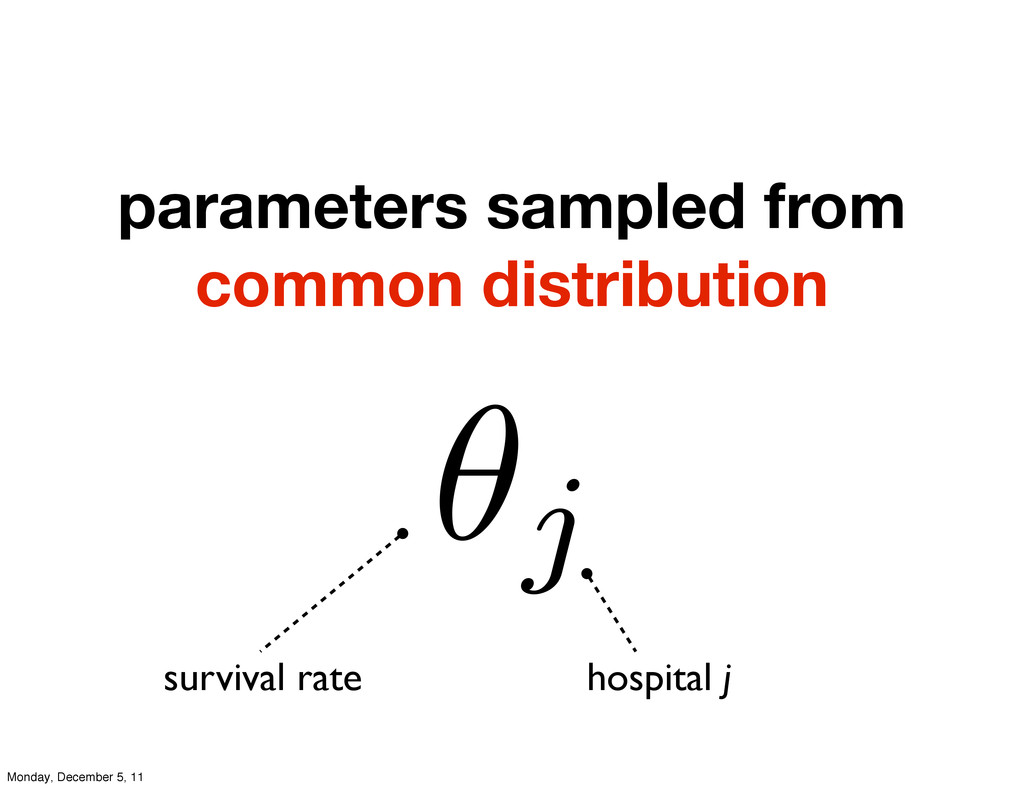
100. parameters sampled from common distribution j hospital j survival rate Monday, December 5, 11
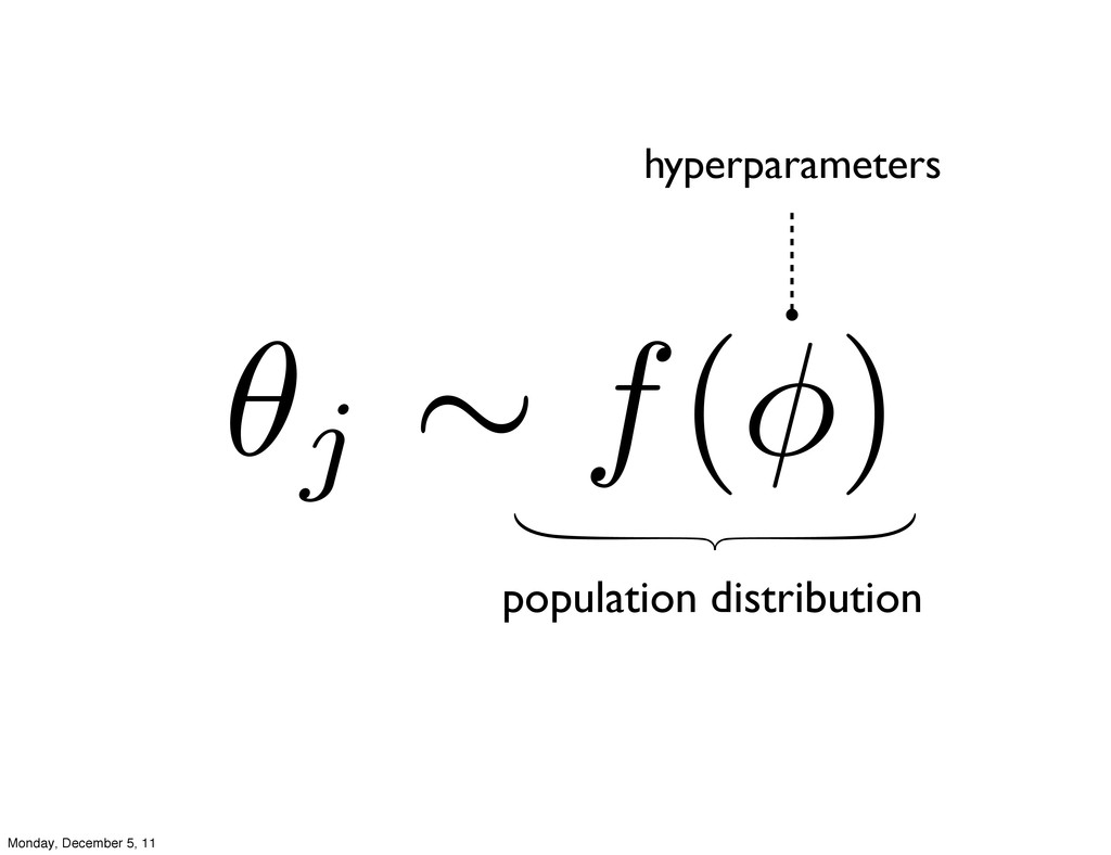
101. population distribution j f(⇥) hyperparameters Monday, December 5, 11
102. θ1 θ2 θk y1 y2 yk ... ... deaths parameters Monday, December 5, 11
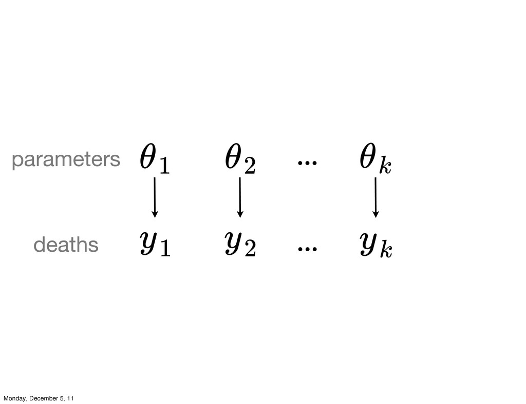
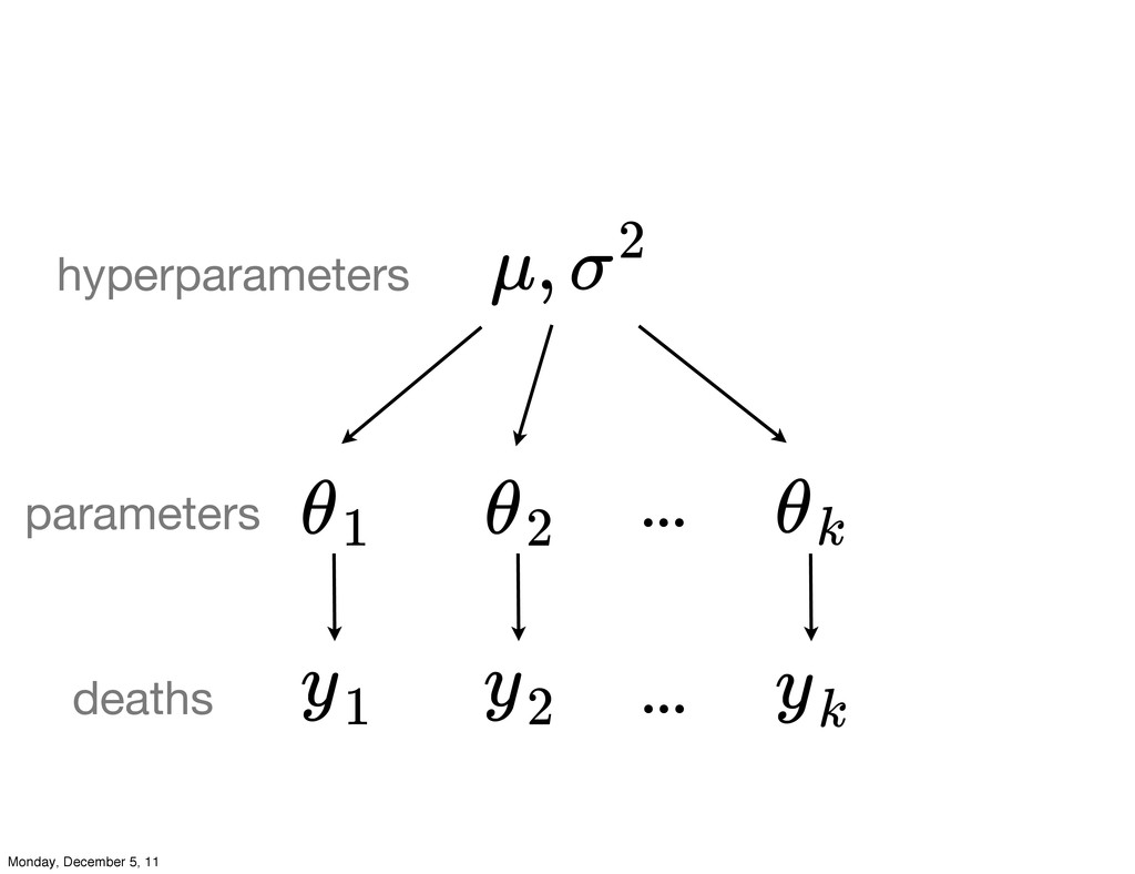
103. θ1 θ2 θk y1 y2 yk ... ... deaths parameters µ, σ2 hyperparameters Monday, December 5, 11
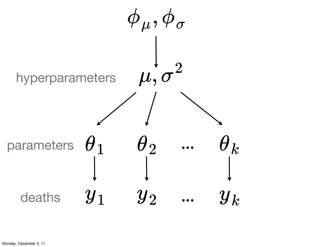
104. , ϕµ ϕσ θ1 θ2 θk y1 y2 yk ... ... deaths parameters µ, σ2 hyperparameters Monday, December 5, 11
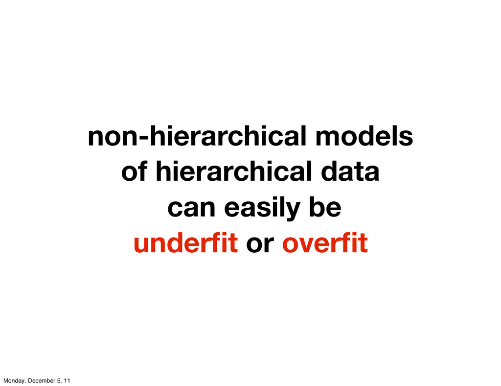
105. non-hierarchical models of hierarchical data can easily be underfit or overfit Monday, December 5, 11
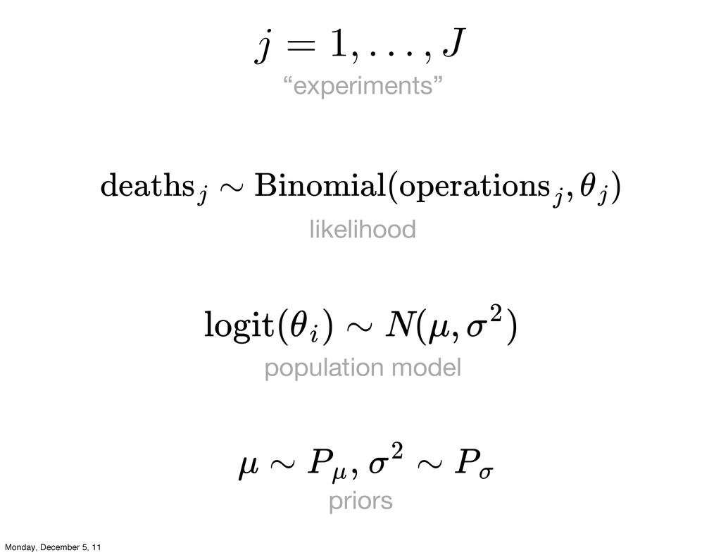
106. “experiments” j = 1, . . . , J likelihood ∼ Binomial( , ) deaths j operations j θj logit( ) ∼ N(µ, ) θi σ2 population model µ ∼ , ∼ Pµ σ2 Pσ priors Monday, December 5, 11
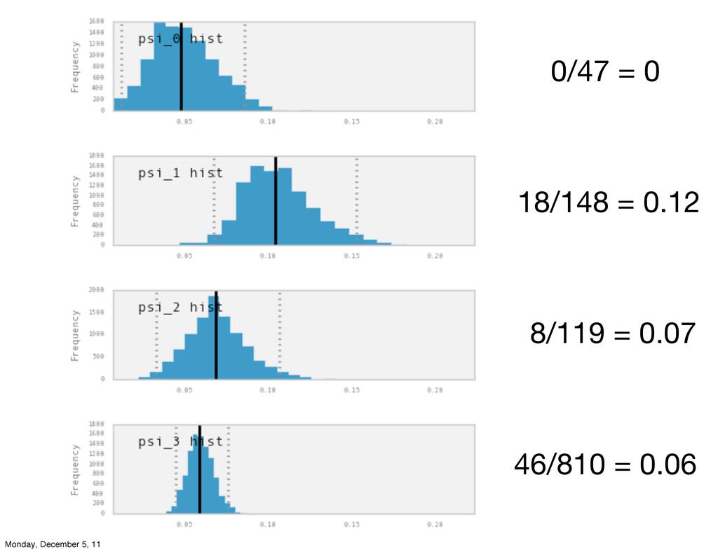
107. 0/47 = 0 18/148 = 0.12 8/119 = 0.07 46/810 = 0.06 Monday, December 5, 11
108. Monday, December 5, 11
109. Monday, December 5, 11