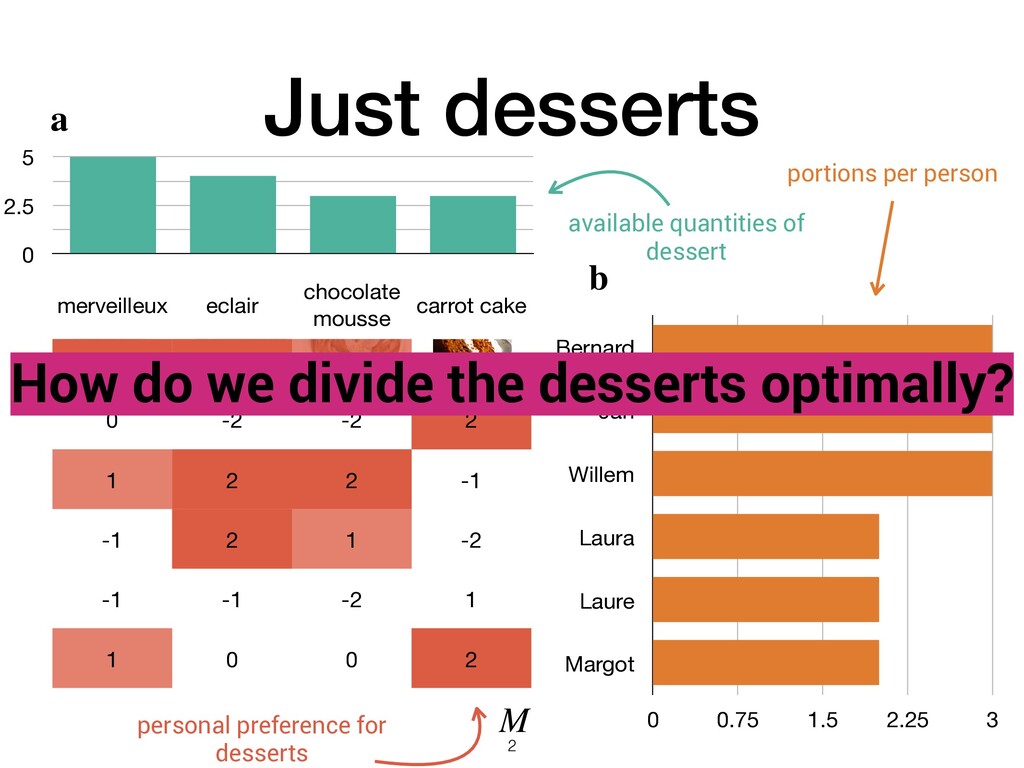
Jan Willem Laura Laure Margot 0 0.75 1.5 2.25 3 portions per person merveilleux eclair chocolate mousse carrot cake 2 2 1 0 0 -2 -2 2 1 2 2 -1 -1 2 1 -2 -1 -1 -2 1 1 0 0 2 personal preference for desserts How do we divide the desserts optimally? a b M 2
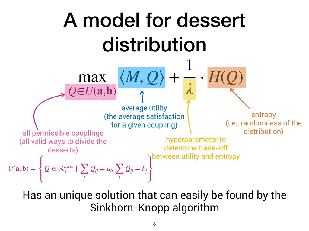
1 λ ⋅ H(Q) average utility (the average satisfaction for a given coupling) hyperparameter to determine trade-off between utility and entropy entropy (i.e., randomness of the distribution) 3 all permissible couplings (all valid ways to divide the desserts) U(a, b) = Q ∈ ℝn×m + ∣ ∑ j Qij = ai , ∑ i Qij = bj Has an unique solution that can easily be found by the Sinkhorn-Knopp algorithm
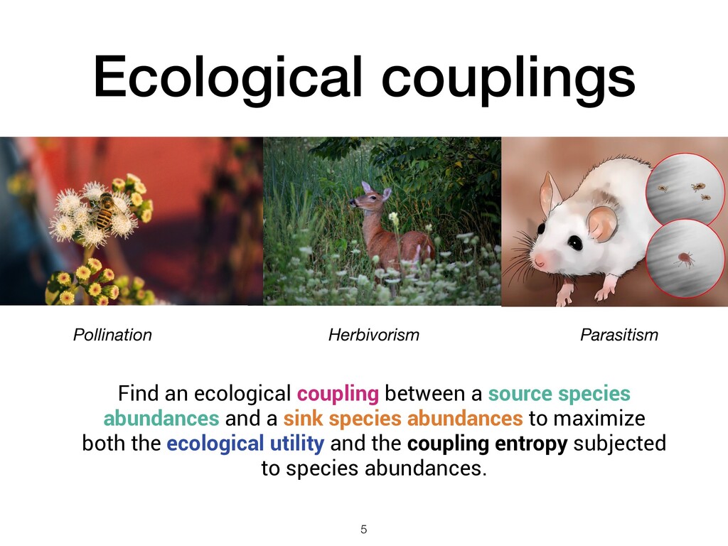
a source species abundances and a sink species abundances to maximize both the ecological utility and the coupling entropy subjected to species abundances. 5
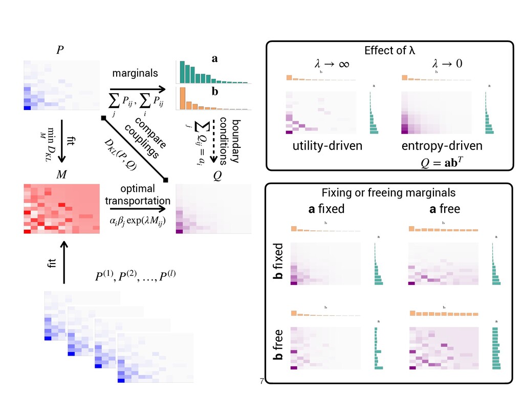
→ ∞ λ → 0 D KL (P,Q ) com pare couplings a b marginals ∑ j Pij , ∑ i Pij boundary conditions optimal transportation αi βj exp(λMij ) ∑ j Qij = ai Q M Fixing or freeing marginals a fixed a free b fixed b free fit min M DKL P(1), P(2), …, P(l) fit 7
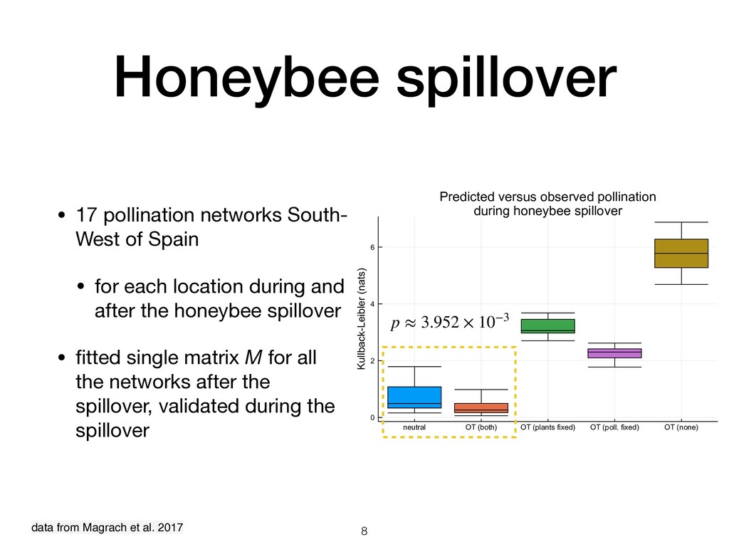
• for each location during and after the honeybee spillover • fitted single matrix M for all the networks after the spillover, validated during the spillover neutral OT (both) OT (plants fixed) OT (poll. fixed) OT (none) 0 2 4 6 Predicted versus observed pollination during honeybee spillover Kullback-Leibler (nats) data from Magrach et al. 2017 p ≈ 3.952 × 10⁻³ 8
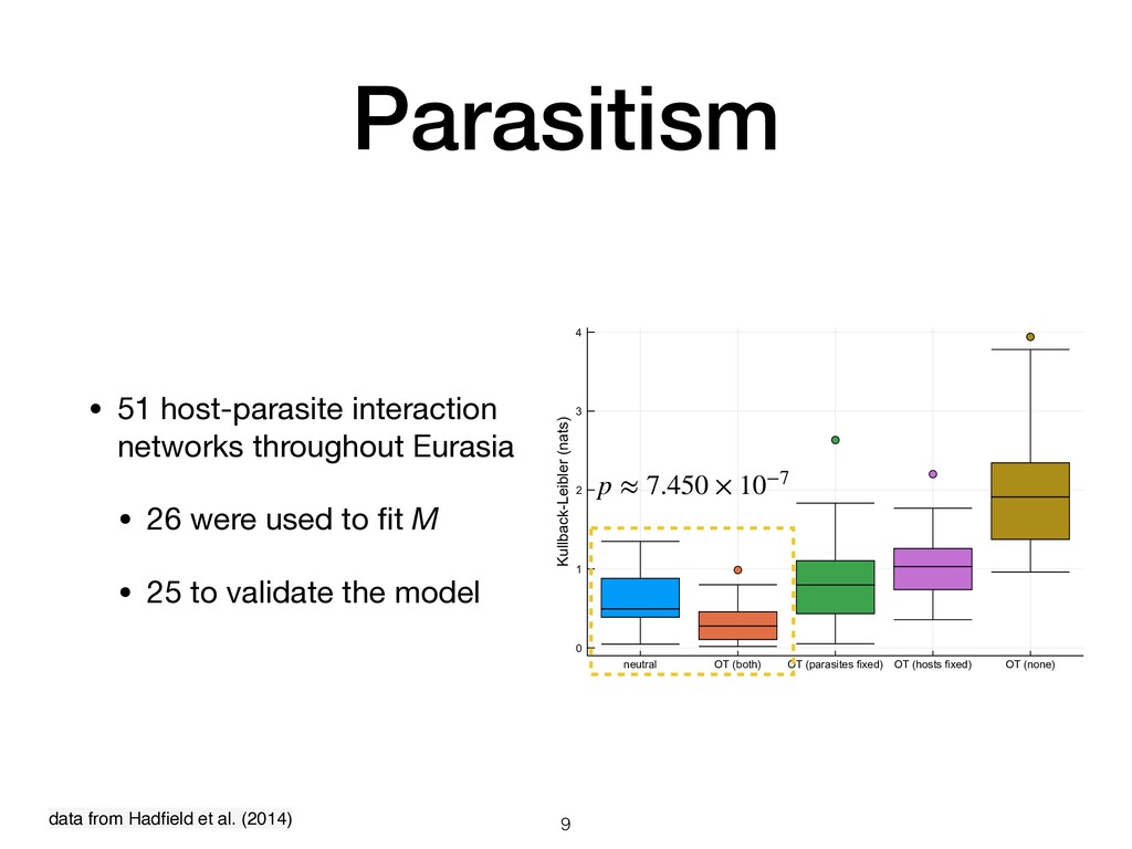
(none) 0 1 2 3 4 Kullback-Leibler (nats) Parasitism • 51 host-parasite interaction networks throughout Eurasia • 26 were used to fit M • 25 to validate the model data from Hadfield et al. (2014) p ≈ 7.450 × 10⁻⁷ 9
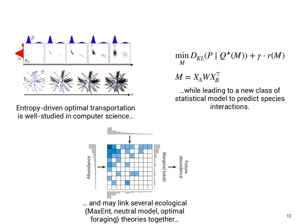
may link several ecological (MaxEnt, neutral model, optimal foraging) theories together… M = XA WX⊤ B min M DKL (P ∣ Q⋆(M)) + γ ⋅ r(M) …while leading to a new class of statistical model to predict species interactions. 10


 michielstock
 rlifchitz
 lychee1223
 konakalab
 yu4u
 hanbao
 trycycle
 neutron63zf
 salt2
 psj59129
 naospon
 ykiyota
 tagtag
 aleyda
 jonoalderson
 madoxten
 lauravandoore
 tmiket
 signer
 portentint
 speakerdeck
 bcantrill
 davidcarrasco
 codingconduct
 schlessera