Tigran Galstyan

(Univ. Paris Saclay, CNRS, CentraleSupélec, L2S)

Title — Statistical and Computational Complexity of the Feature Matching Map Detection Problem

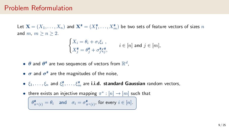
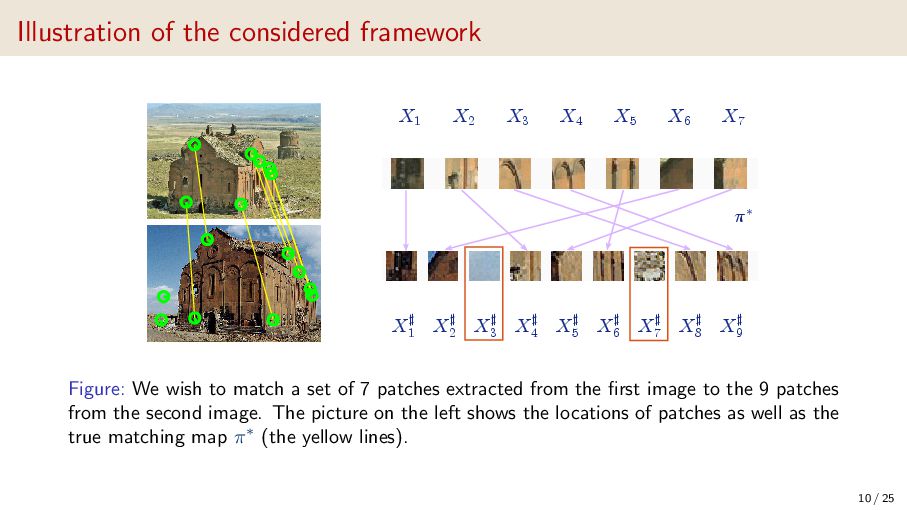
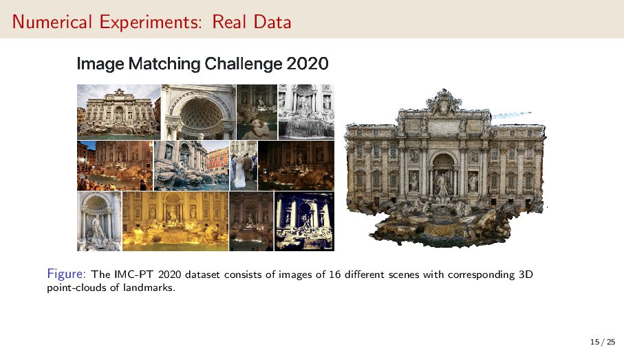
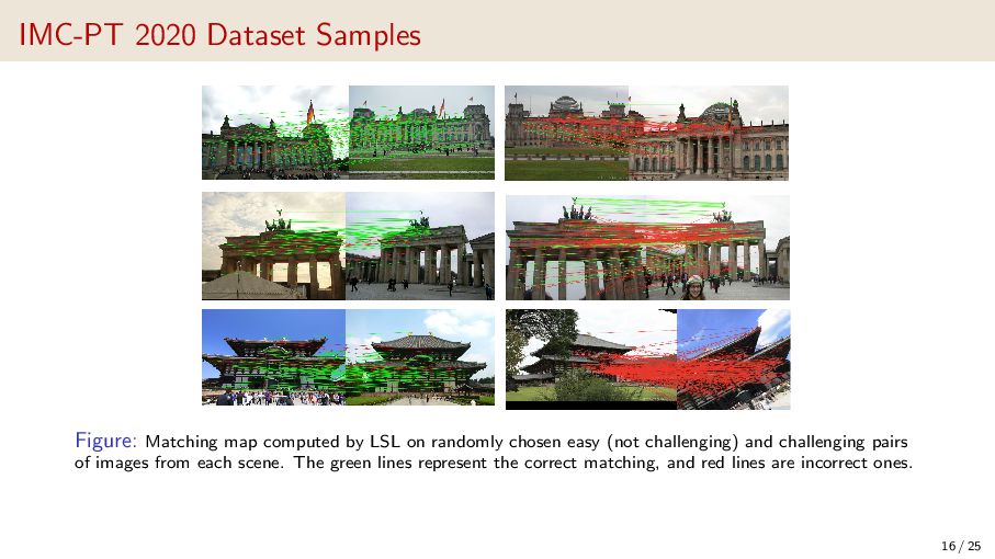
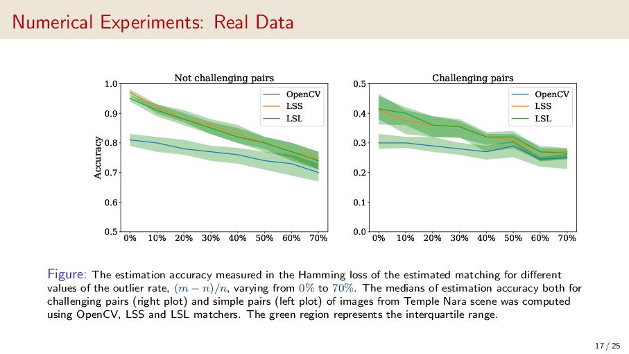
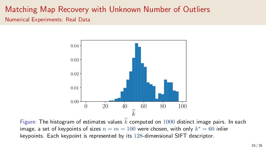
Abstract — The problem of finding the best matching between two point clouds has been extensively studied, both theoretically and experimentally. The matching problem arises in various applications, for instance in computer vision, bioinformatics and natural language processing. In computer vision, finding the correspondence between two sets of local descriptors extracted from two images of the same scene is a well-known example of a matching problem. When datasets do not contain outliers, meaning that both matching sets have the same size and all points have their corresponding match in the other dataset, the optimality of the matching procedures was previously studied from a minimax statistical viewpoint. Clearly, in aforementioned applications, not all the points have their matching point and one can hardly know in advance how many points have their corresponding matching points. This work focuses on various extended settings of the problem (i.e. containing outliers) and gaining a theoretical understanding of the statistical limitations of the matching problem.

Transcript

1. Statistical and Computational Complexity of the Feature Matching Map Detection Problem Tigran Galstyan Postdoctoral researcher CNRS, CentraleSup´ elec S3 The Paris-Saclay Signal and Statistics Seminar October 17, 2025 1 / 25
2. Introduction • Establishing a correspondence, or matching, between two sets of data is a fundamental challenge that appears in numerous domains. • In computer vision, a classic example is matching local feature descriptors across two images of the same scene, a critical step for tasks like 3D reconstruction and panoramic stitching. • In computational biology, matching entities from different single-cell datasets is essential for creating a unified and enhanced view of cellular processes. • In Natural Language Processing, matching is central to semantic search and Retrieval-Augmented Generation (RAG), where a user’s query is matched against a vector database to retrieve relevant documents that provide context for a Large Language Model. The goal of the present work is to gain a theoretical understanding of the statistical limits of this fundamental feature matching problem. 2 / 25
3. Real Life Example Figure: An example from IMC-PT 2020 image matching dataset. 3 / 25
4. Mathematical formulation of the problem • Notation: [n] = {1, . . . , n} for any positive integer n and ∥ · ∥ the Euclidean norm in Rd • Assume two independent sequences X = (Xi; i ∈ [n]) and Y = (Yi; i ∈ [n]) of independent vectors, such that Xi, Yi ∼ Pi on Rd. • We observe X and X# - a shuffled version of Y . • That is X# i = Yπ∗(i) for some unobserved permutation π∗. • The goal is to recover the π∗ from data (X, X#). We consider the simplest case Pi = Nd(θi, σ2 i Id), leading to    Xi = θi + σiξi , X# i = θ# i + σ# i ξ# i , i = 1, . . . , n and θ# π∗(i) = θi 4 / 25
5. Mathematical formulation of the problem Let X = (X1, . . . , Xn) and X# = (X# 1 , . . . , X# n ) be two sets of feature vectors of size n.    Xi = θi + σiξi , X# i = θ# i + σ# i ξ# i , i = 1, . . . , n and θ# π∗(i) = θi (1) • θ = (θ1, . . . , θn) and θ# = (θ# 1 , . . . , θ# n ) are two sequences of vectors from Rd, which are unavailable, • σ = (σ1, . . . , σn)⊤, σ# = (σ# 1 , . . . , σ# n )⊤ the magnitudes of the noise contaminating each feature, • ξ1, . . . , ξn and ξ# 1 , . . . , ξ# n are two independent sequences of i.i.d. standard Gaussian random vectors, • there exists a bijective mapping π∗ : [n] → [n] such that θi = θ# π∗(i) for all i ∈ [n]. 5 / 25
6. Useful Concepts • Our ultimate goal is to design estimators that will exactly recover the matching π∗ with prescribed high probability ( P(π = π∗) ≥ 1 − α. ) under the weakest possible conditions on the nuisance parameters (θ, θ#) and (σ, σ#). • Detection of the matching is harder when the feature vectors are close. To quantify this phenomenon, we introduce the separation distance κ, which measures minimal distance-to-noise ratio. The precise definition is: κ = min i̸=j ∥θi − θj∥ (σ2 i + σ2 j )1/2 . 6 / 25
7. Prior Work Collier, O. and Dalalyan, A. “Minimax rates in permutation estimation for feature matching.” The Journal of Machine Learning Research, 2016, 17(1), 162-192. • The LSL (Least Sum of Logarithms) estimator πLSL ∈ arg min π:[n]→[n] i∈[n] log ∥Xi − X# π(i) ∥2 2 . is minimax optimal for exact permutation recovery. • The minimax optimal rate is κ ∝ d log(n2/α) 1/4 ∨ log(n2/α)1/2 . • This problem, also called the “assignment problem”, can be solved using the Hungarian algorithm with O(n3) computational complexity. 7 / 25
8. Outliers in one of the sets. Galstyan, T., Minasyan, A., and Dalalyan, A. ”Optimal detection of the feature matching map in presence of noise and outliers.” Electronic Journal of Statistics, 2022, 16(2), 5720-5750. 8 / 25
9. Problem Reformulation Let X = (X1 , . . . , Xn ) and X# = (X# 1 , . . . , X# m ) be two sets of feature vectors of sizes n and m, m ≥ n ≥ 2. Xi = θi + σi ξi , X# j = θ# j + σ# j ξ# j , i ∈ [n] and j ∈ [m], • θ and θ# are two sequences of vectors from Rd, • σ and σ# are the magnitudes of the noise, • ξ1 , . . . , ξn and ξ# 1 , . . . , ξ# m are i.i.d. standard Gaussian random vectors, • there exists an injective mapping π∗ : [n] → [m] such that θ# π∗(i) = θi and σi = σ# π∗(i) , for every i ∈ [n]. 9 / 25
10. Illustration of the considered framework :$ X1 X2 X3 X4 X5 X6 X7 X] 1 X] 2 X] 3 X] 4 X] 5 X] 6 X] 7 X] 8 X] 9 Figure: We wish to match a set of 7 patches extracted from the first image to the 9 patches from the second image. The picture on the left shows the locations of patches as well as the true matching map π∗ (the yellow lines). 10 / 25
11. Separation Distances We introduce the separation distance ¯ κin-in = ¯ κin-in(θ#, σ#, π∗) and the outlier separation distance ¯ κin-out = ¯ κin-out(θ#, σ#, π∗). The precise definitions read as: ¯ κin-in ≜ min i,j̸∈Oπ∗ , j̸=i ∥θ# i − θ# j ∥ (σ# i 2 + σ# j 2)1/2 , ¯ κin-out ≜ min i̸∈Oπ∗ , j∈Oπ∗ ∥θ# i − θ# j ∥ (σ# i 2 + σ# j 2)1/2 . (1) where Oπ∗ ≜ [m] \ Im(π∗). 11 / 25
12. Upper bound for LSL πLSL n,m ≜ arg min π:[n]→[m] n i=1 log ∥Xi − X# π(i) ∥2, Theorem (Upper bound for LSL) Let α ∈ (0, 1/2). If the separation distances ¯ κin-in and ¯ κin-out corresponding to (θ#, σ#, π∗) and defined by (1) satisfy min{¯ κin-in, ¯ κin-out} ≥ √ 2d + 4 2d log(4nm/α) 1/4 ∨ 3 log(8nm/α 1/2 then the LSL estimator detects the matching map π∗ with probability at least 1 − α, that is Pθ#,σ#,π∗ (πLSL n,m = π∗) ≥ 1 − α. 12 / 25
13. Summary of the Results Without outliers With outliers current work unknown σ# σmax/σmin ≤ C unknown σ# arbitrary LSL is optimal ¯ κ ≳ (d log n)1/4 LSL is optimal ¯ κin-in ≳ (d log(nm))1/4 & ¯ κin-out ≳ d1/2 LSL is optimal ¯ κin-in ∧ ¯ κin-out ≳ d1/2 • The table shows results in the high-dimensional regime d ≥ c log n. • Given rates for ¯ κ are minimax optimal. • Presence of outliers makes the statistical problem significantly harder. • Limiting σmax/σmin enables us to achieve separate rates for ¯ κin-in and ¯ κin-out . 13 / 25
14. Numerical Experiments: Synthetic Data Figure: The performance of the methods (Greedy, LSS, LSL, LSNS). Curves represent the error rates as a function of separation distances. The picture illustrates that LSS, LSL and LSNS require much lower value of ¯ κin-in in order to find the correct matching map. 14 / 25
15. Numerical Experiments: Real Data Figure: The IMC-PT 2020 dataset consists of images of 16 different scenes with corresponding 3D point-clouds of landmarks. 15 / 25
16. IMC-PT 2020 Dataset Samples Figure: Matching map computed by LSL on randomly chosen easy (not challenging) and challenging pairs of images from each scene. The green lines represent the correct matching, and red lines are incorrect ones. 16 / 25
17. Numerical Experiments: Real Data 0% 10% 20% 30% 40% 50% 60% 70% 0.5 0.6 0.7 0.8 0.9 1.0 Accuracy Not challenging pairs OpenCV LSS LSL 0% 10% 20% 30% 40% 50% 60% 70% 0.0 0.1 0.2 0.3 0.4 0.5 Challenging pairs OpenCV LSS LSL Figure: The estimation accuracy measured in the Hamming loss of the estimated matching for different values of the outlier rate, (m − n)/n, varying from 0% to 70%. The medians of estimation accuracy both for challenging pairs (right plot) and simple pairs (left plot) of images from Temple Nara scene was computed using OpenCV, LSS and LSL matchers. The green region represents the interquartile range. 17 / 25
18. Outliers present in both sets. Minasyan, A., Galstyan, T., Hunanyan, S. and Dalalyan, A., ”Matching map recovery with an unknown number of outliers.” In International Conference on Artificial Intelligence and Statistics (pp. 891-906). PMLR. 2023. 18 / 25
19. Problem Reformulation Let X = (X1 , . . . , Xn ) and X# = (X# 1 , . . . , X# m ) be two sets of feature vectors of sizes n and m, m ≥ n ≥ 2. Xi = θi + σξi , X# j = θ# j + σ#ξ# j , i ∈ [n] and j ∈ [m], • θ and θ# are two sequences of vectors from Rd, • ξ1 , . . . , ξn , ξ# 1 , . . . , ξ# m i.i.d. ∼ N(0, Id ), For some S∗ ⊂ [n] of cardinality k∗ ≤ n, there exists an injective mapping π∗ : S∗ → [m] such that θi = θ# π∗(i) holds for all i ∈ S∗. 19 / 25
20. Definitions We redefine signal-to-noise ratio as follows: κi,j = ∥θi − θ# j ∥2 /(σ2 + σ#2)1/2, ¯ κall ≜ min i∈[n] min j∈[m]\{π∗(i)} κi,j Pk is the set of all k-matching maps: Pk := π : S → [m] such that S ⊂ [n], |S| = k, π is injective We define πLSS k as the solution to the following optimization problem and Φ(k) as its error: πLSS k ∈ arg min π∈Pk i∈Sπ ∥Xi − X# π(i) ∥2 2 , Φ(k) = min π∈Pk i∈Sπ ∥Xi − X# π(i) ∥2 2 . where Sπ denotes the support of function π. 20 / 25
21. Summary of Theoretical Results • If ¯ κall ≳ d log(nm α ) 1/4 ∨ log(nm α ) 1/2 and the value of k is smaller than k∗, we prove that πLSS k makes no mistake with probability 1 − α. • We design a data-driven model selection algorithm that adaptively chooses k such that with probability 1 − α, we have k = k∗ and πLSS k = π∗ whenever ¯ κall ≳ d log(nm α ) 1/4 ∨ log(nm α ) 1/2. 21 / 25
22. Main Algorithm • To compute each Φ(k) we need to solve the optimization problem from scratch. • Φ is strictly increasing. • kmin is optional (for time efficiency), can be set to kmin = 1. 22 / 25
23. Relation to Minimum Cost Flow Problem X1 X2 X3 X4 X# 1 X# 2 X# 3 X# 4 X# 5 src sink X X# d1,1 d2,1 d3,5 Figure: Matching as a Minimum Cost Flow (MCF) problem. The idea is to augment the graph with two nodes, source and sink, and n + m edges. The capacities of orange edges should be set to 1, while the cost should be set to 0. Setting the total flow sent through the graph to k, the solution of the MCF becomes a matching of size k. 23 / 25
24. Numerical Experiments: Synthetic Data Figure: The top plot shows the dependence of the estimate of k∗ on ¯ κall , while the bottom one—the dependence of the estimate of σ2 0 on ¯ κall . 24 / 25
25. Thank You! 25 / 25
26. Lower bound We will say that an estimator πn of π∗ is a distance based M-estimator, if for a sequence of non-decreasing functions ρi : R+ → R, i = 1, . . . , n, the following is correct πn ∈ arg min π:[n]→[m] n i=1 ρi ∥Xi − X# π(i) ∥ , We denote by M the set of all distance based M-estimators. We show that there is indeed a setup where ¯ κin-in ∧ ¯ κin-out is as large as 0.2 √ d but any estimator from M fails to detect π∗ with probability at least 1/4. 25 / 25
27. Lower bound Theorem (Lower bound over M) Assume that m > n ≥ 4 and d ≥ 422 log(4n). There exists a triplet (σ#, θ#, π∗) such that ¯ κin-in = ¯ κin-out = d/20 and inf π∈M Pθ#,σ#,π∗ (π ̸= π∗) > 1/4. Theorem (General lower bound) Denote κ = min{¯ κin-in, ¯ κin-out}. Assume that m > n ≥ 5 and d ≥ 16 log(nm). Then, there exists a triplet (σ#, θ#, π∗) such that 6κ ≥ (d log(nm))1/4 and inf π Pθ#,σ#,π∗ (π ̸= π∗) > 1/3, where the infimum is taken over all injective matching maps π : [n] → [m]. 25 / 25
28. Matching Map Recovery with Unknown Number of Outliers Numerical Experiments: Real Data Figure: For illustration purposes, we have selected 3 scenarios. In the top-left plot n = 50 and k∗ = 25. Algorithm 1 outputs k = 22 and πLSS k = π∗ (perfect matching). In the top-right plot n = 100 and k∗ = 50, the estimated value of k∗ is k = 44. In the bottom plot we selected n = 350 keypoints from which k∗ = 250 were inliers (k = 213). In all scenarios matching map contained only few mistakes. 25 / 25
29. Matching Map Recovery with Unknown Number of Outliers Numerical Experiments: Real Data 0 20 40 60 80 100 k 0.00 0.01 0.02 0.03 0.04 Figure: The histogram of estimates values k computed on 1000 distinct image pairs. In each image, a set of keypoints of sizes n = m = 100 were chosen, with only k∗ = 60 inlier keypoints. Each keypoint is represented by its 128-dimensional SIFT descriptor. 25 / 25