Kernels and Support Vector Machines

* Kernel Families
* Support Vector Machines

Transcript

1. Seminar 2 Kernels and Support Vector Machines Edgar Marca Supervisor: DSc. André M.S. Barreto Petrópolis, Rio de Janeiro - Brazil September 2nd, 2015 1 / 28
2. Kernels
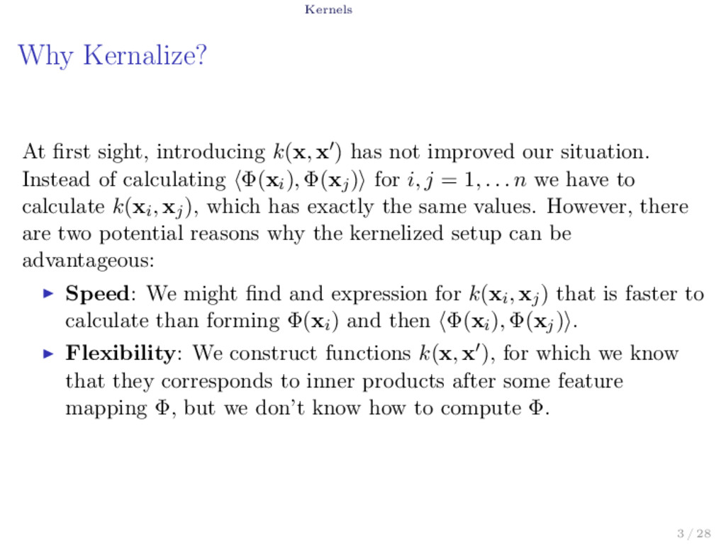
3. Kernels Why Kernalize? At first sight, introducing k(x, x′) has not improved our situation. Instead of calculating ⟨Φ(xi), Φ(xj)⟩ for i, j = 1, . . . n we have to calculate k(xi, xj), which has exactly the same values. However, there are two potential reasons why the kernelized setup can be advantageous: ▶ Speed: We might find and expression for k(xi, xj) that is faster to calculate than forming Φ(xi) and then ⟨Φ(xi), Φ(xj)⟩. ▶ Flexibility: We construct functions k(x, x′), for which we know that they corresponds to inner products after some feature mapping Φ, but we don’t know how to compute Φ. 3 / 28
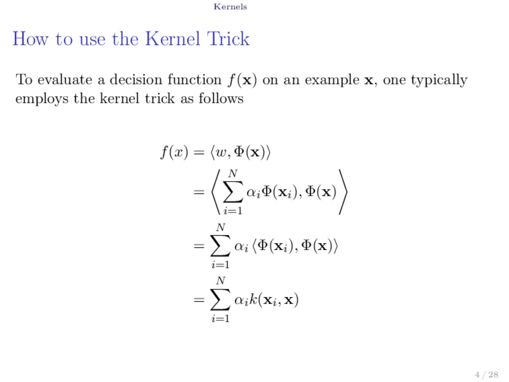
4. Kernels How to use the Kernel Trick To evaluate a decision function f(x) on an example x, one typically employs the kernel trick as follows f(x) = ⟨w, Φ(x)⟩ = ⟨ N ∑ i=1 αiΦ(xi), Φ(x) ⟩ = N ∑ i=1 αi ⟨Φ(xi), Φ(x)⟩ = N ∑ i=1 αik(xi, x) 4 / 28
5. How to proof that a function is a kernel?
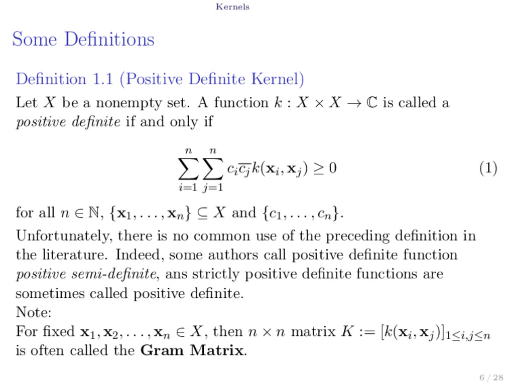
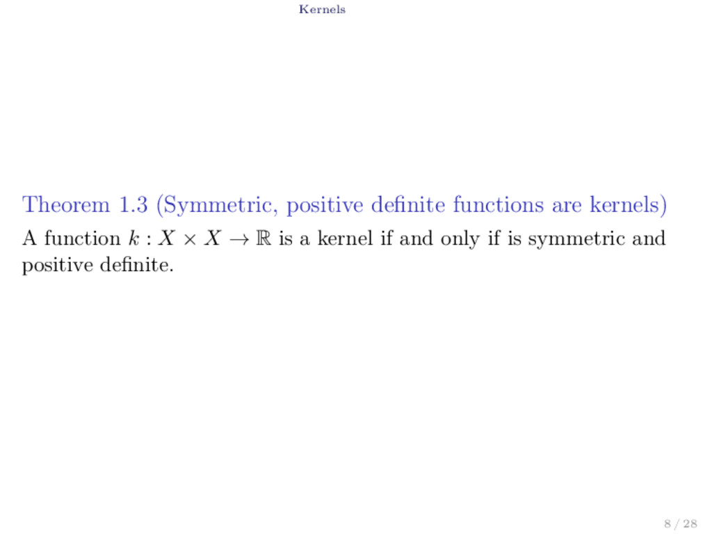
6. Kernels Some Definitions Definition 1.1 (Positive Definite Kernel) Let X be a nonempty set. A function k : X × X → C is called a positive definite if and only if n ∑ i=1 n ∑ j=1 cicjk(xi, xj) ≥ 0 (1) for all n ∈ N, {x1, . . . , xn} ⊆ X and {c1, . . . , cn}. Unfortunately, there is no common use of the preceding definition in the literature. Indeed, some authors call positive definite function positive semi-definite, ans strictly positive definite functions are sometimes called positive definite. Note: For fixed x1, x2, . . . , xn ∈ X, then n × n matrix K := [k(xi, xj)]1≤i,j≤n is often called the Gram Matrix. 6 / 28
7. Kernels Mercer Condition Theorem 1.2 Let X = [a, b] be compact interval and let k : [a, b] × [a, b] → C be continuous. Then φ is positive definite if and only if ∫ b a ∫ b a c(x)c(y)k(x, y)dxdy ≥ 0 (2) for each continuous function c : X → C. 7 / 28
8. Kernels Theorem 1.3 (Symmetric, positive definite functions are kernels) A function k : X × X → R is a kernel if and only if is symmetric and positive definite. 8 / 28
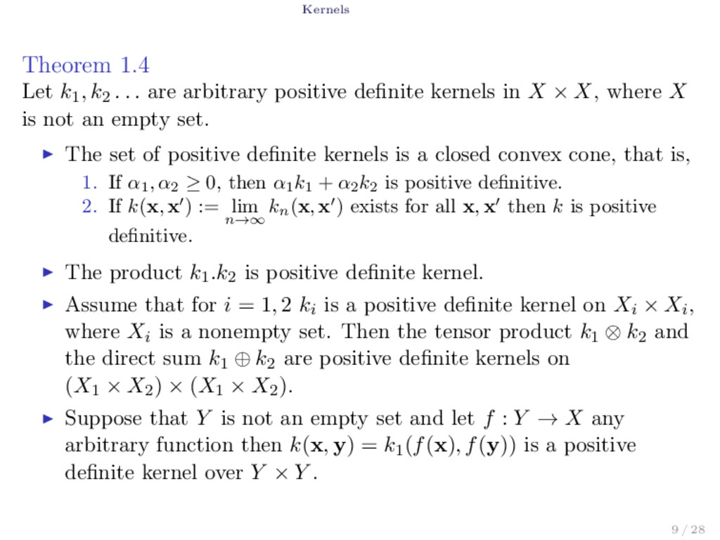
9. Kernels Theorem 1.4 Let k1, k2 . . . are arbitrary positive definite kernels in X × X, where X is not an empty set. ▶ The set of positive definite kernels is a closed convex cone, that is, 1. If α1 , α2 ≥ 0, then α1 k1 + α2 k2 is positive definitive. 2. If k(x, x′) := lim n→∞ kn (x, x′) exists for all x, x′ then k is positive definitive. ▶ The product k1.k2 is positive definite kernel. ▶ Assume that for i = 1, 2 ki is a positive definite kernel on Xi × Xi, where Xi is a nonempty set. Then the tensor product k1 ⊗ k2 and the direct sum k1 ⊕ k2 are positive definite kernels on (X1 × X2) × (X1 × X2). ▶ Suppose that Y is not an empty set and let f : Y → X any arbitrary function then k(x, y) = k1(f(x), f(y)) is a positive definite kernel over Y × Y . 9 / 28
10. Kernel Families
11. Kernels Kernel Families Translation Invariant Kernels Definition 1.5 A translation invariant kernel is given by K(x, y) = k(x − y) (3) where k is a even function in Rn, i.e., k(−x) = k(x) for all x in Rn. 11 / 28
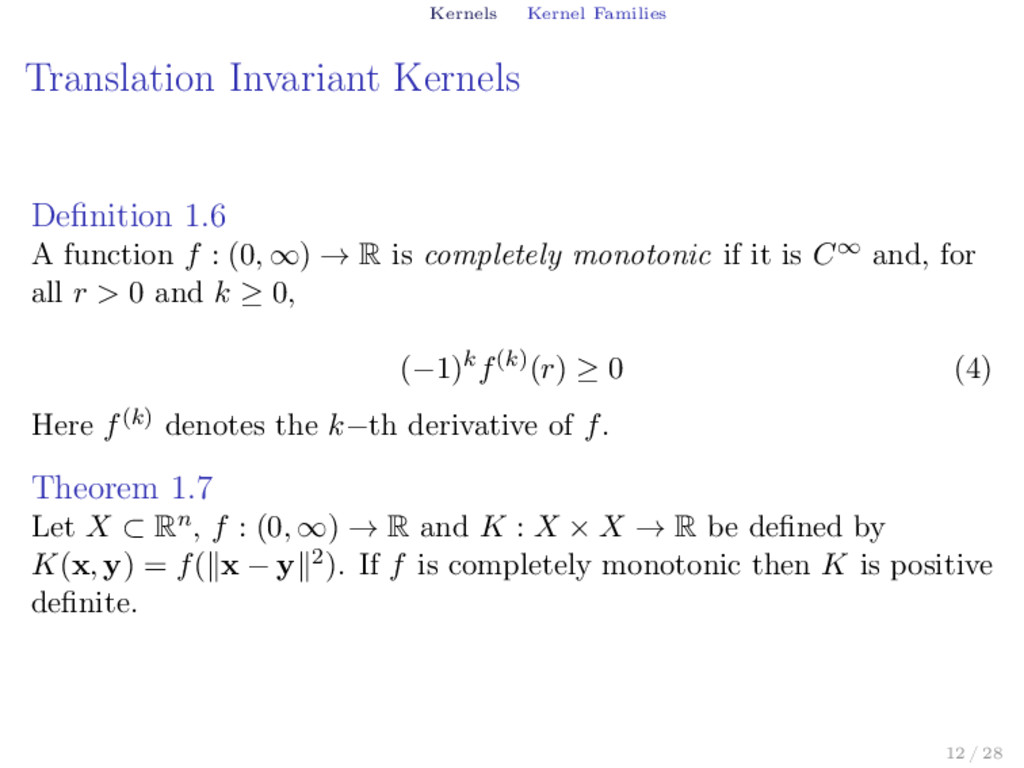
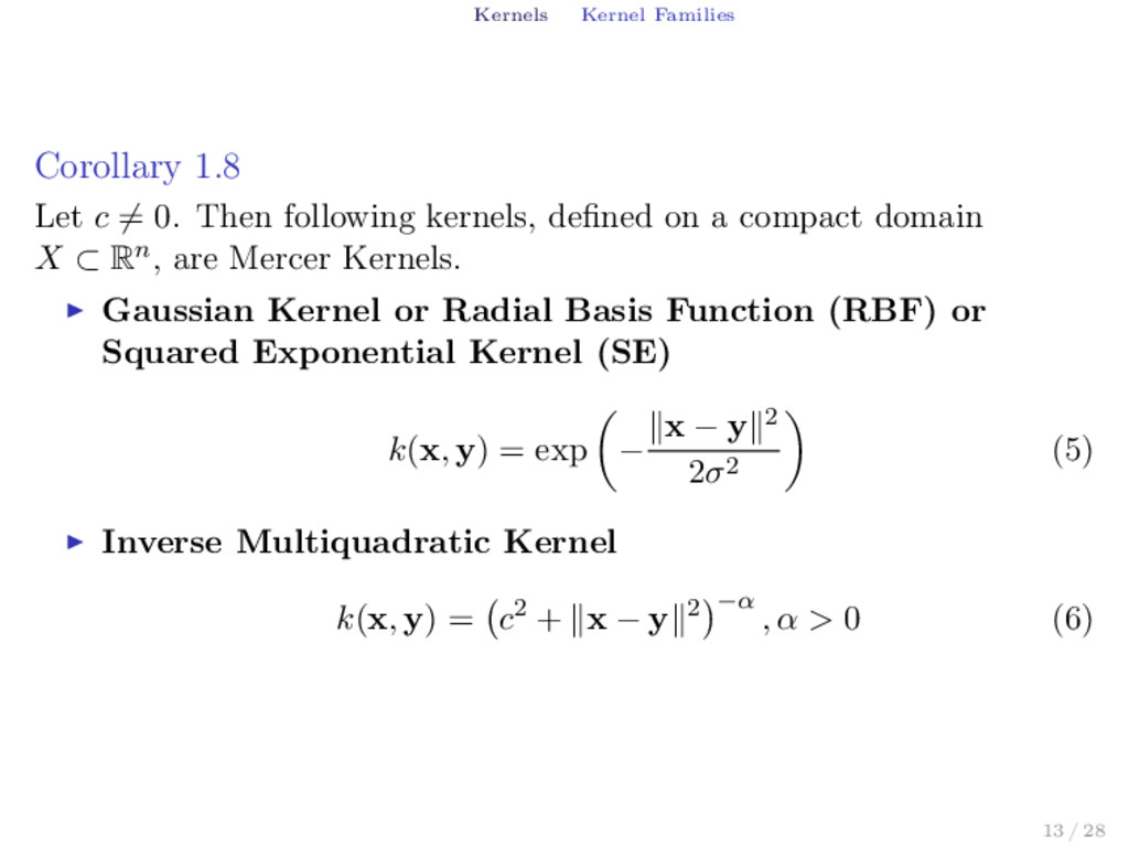
12. Kernels Kernel Families Translation Invariant Kernels Definition 1.6 A function f : (0, ∞) → R is completely monotonic if it is C∞ and, for all r > 0 and k ≥ 0, (−1)kf(k)(r) ≥ 0 (4) Here f(k) denotes the k−th derivative of f. Theorem 1.7 Let X ⊂ Rn, f : (0, ∞) → R and K : X × X → R be defined by K(x, y) = f(∥x − y∥2). If f is completely monotonic then K is positive definite. 12 / 28
13. Kernels Kernel Families Corollary 1.8 Let c ̸= 0. Then following kernels, defined on a compact domain X ⊂ Rn, are Mercer Kernels. ▶ Gaussian Kernel or Radial Basis Function (RBF) or Squared Exponential Kernel (SE) k(x, y) = exp ( − ∥x − y∥2 2σ2 ) (5) ▶ Inverse Multiquadratic Kernel k(x, y) = ( c2 + ∥x − y∥2 )−α , α > 0 (6) 13 / 28
14. Kernels Kernel Families Polynomial Kernels k(x, x′) = (α⟨x, x′⟩ + c)d, α > 0, c ≥ 0, d ∈ Z (7) 14 / 28
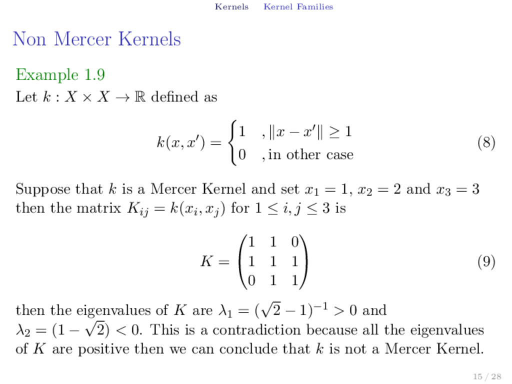
15. Kernels Kernel Families Non Mercer Kernels Example 1.9 Let k : X × X → R defined as k(x, x′) = { 1 , ∥x − x′∥ ≥ 1 0 , in other case (8) Suppose that k is a Mercer Kernel and set x1 = 1, x2 = 2 and x3 = 3 then the matrix Kij = k(xi, xj) for 1 ≤ i, j ≤ 3 is K =   1 1 0 1 1 1 0 1 1   (9) then the eigenvalues of K are λ1 = ( √ 2 − 1)−1 > 0 and λ2 = (1 − √ 2) < 0. This is a contradiction because all the eigenvalues of K are positive then we can conclude that k is not a Mercer Kernel. 15 / 28
16. Kernels Kernel Families References for Kernels [3] C. Berg, J. Reus, and P. Ressel. Harmonic Analysis on Semigroups: Theory of Positive Definite and Related Functions. Springer Science+Business Media, LLV, 1984. [9] Felipe Cucker and Ding Xuan Zhou. Learning Theory. Cambridge University Press, 2007. [47] Ingo Steinwart and Christmannm Andreas. Support Vector Machines. 2008. 16 / 28
17. Support Vector Machines
18. Applications SVM Support Vector Machines w, x + b = 1 w, x + b = −1 w, x + b = 0 margen Figure: Linear Support Vector Machine 18 / 28
19. Applications SVM Primal Problem Theorem 3.1 The optimization program for the maximum margin classifier is    min w,b 1 2 ∥w∥2 s.a yi(⟨w, xi⟩ + b) ≥ 1, ∀i, 1 ≤ i ≤ m (10) 19 / 28
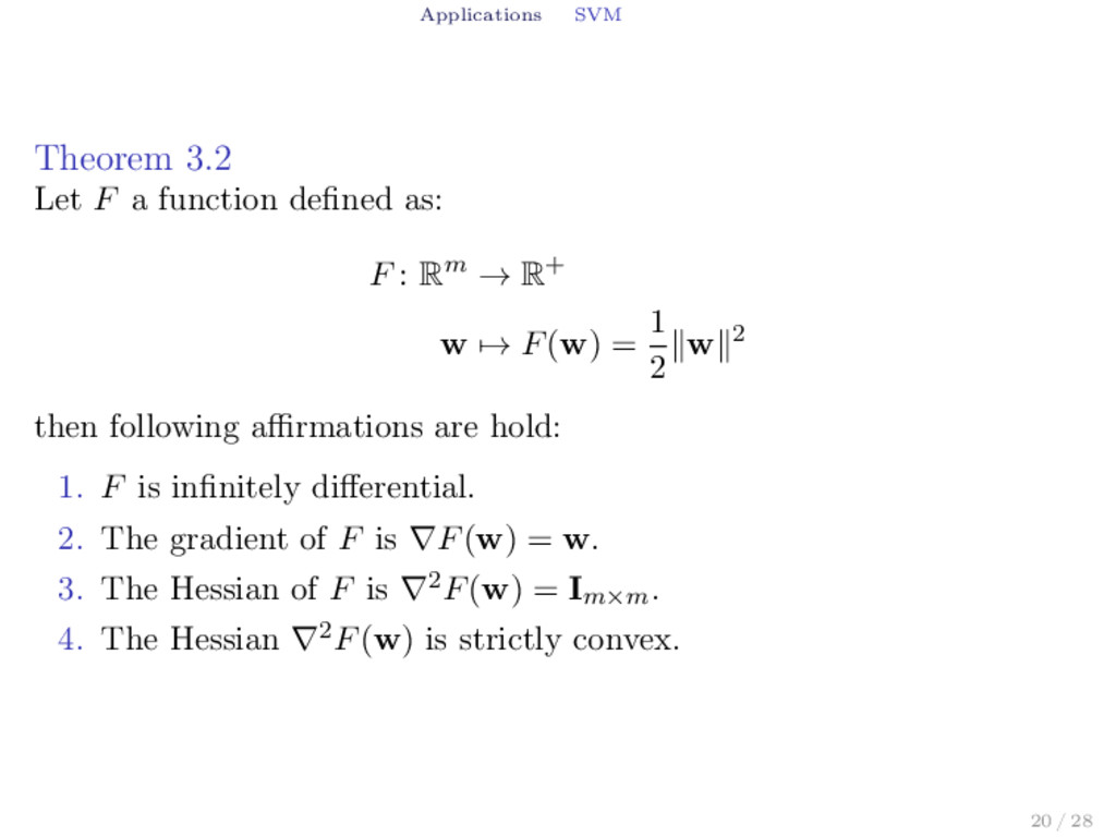
20. Applications SVM Theorem 3.2 Let F a function defined as: F : Rm → R+ w → F(w) = 1 2 ∥w∥2 then following affirmations are hold: 1. F is infinitely differential. 2. The gradient of F is ∇F(w) = w. 3. The Hessian of F is ∇2F(w) = Im×m. 4. The Hessian ∇2F(w) is strictly convex. 20 / 28
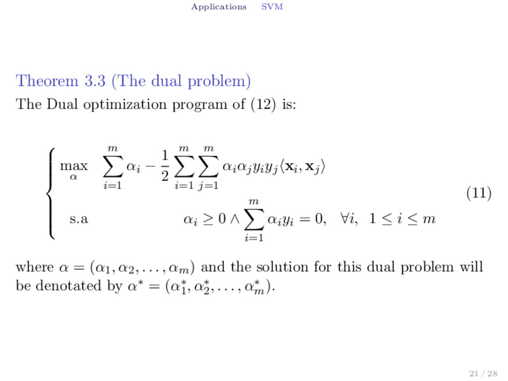
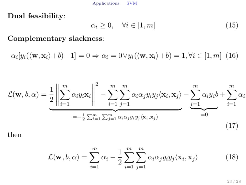
21. Applications SVM Theorem 3.3 (The dual problem) The Dual optimization program of (12) is:            max α m ∑ i=1 αi − 1 2 m ∑ i=1 m ∑ j=1 αiαjyiyj⟨xi, xj⟩ s.a αi ≥ 0 ∧ m ∑ i=1 αiyi = 0, ∀i, 1 ≤ i ≤ m (11) where α = (α1, α2, . . . , αm) and the solution for this dual problem will be denotated by α∗ = (α∗ 1 , α∗ 2 , . . . , α∗ m ). 21 / 28
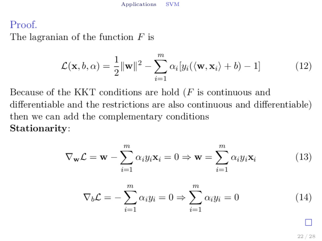
22. Applications SVM Proof. The lagranian of the function F is L(x, b, α) = 1 2 ∥w∥2 − m ∑ i=1 αi[yi(⟨w, xi⟩ + b) − 1] (12) Because of the KKT conditions are hold (F is continuous and differentiable and the restrictions are also continuous and differentiable) then we can add the complementary conditions Stationarity: ∇wL = w − m ∑ i=1 αiyixi = 0 ⇒ w = m ∑ i=1 αiyixi (13) ∇bL = − m ∑ i=1 αiyi = 0 ⇒ m ∑ i=1 αiyi = 0 (14) 22 / 28
23. Applications SVM Primal feasibility: yi(⟨w, xi⟩ + b) ≥ 1, ∀i ∈ [1, m] (15) Dual feasibility: αi ≥ 0, ∀i ∈ [1, m] (16) Complementary slackness: αi[yi(⟨w, xi⟩+b)−1] = 0 ⇒ αi = 0∨yi(⟨w, xi⟩+b) = 1, ∀i ∈ [1, m] (17) L(w, b, α) = 1 2 m ∑ i=1 αiyixi 2 − m ∑ i=1 m ∑ j=1 αiαjyiyj⟨xi, xj⟩ =− 1 2 ∑ m i=1 ∑ m j=1 αiαjyiyj⟨xi,xj⟩ − m ∑ i=1 αiyib =0 + m ∑ i=1 αi (18) then L(w, b, α) = m ∑ i=1 αi − 1 2 m ∑ i=1 m ∑ j=1 αiαjyiyj⟨xi, xj⟩ (19) 23 / 28
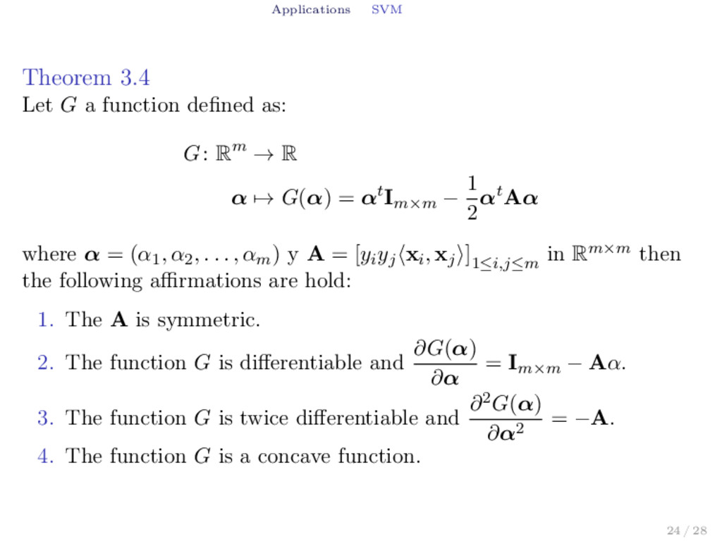
24. Applications SVM Theorem 3.4 Let G a function defined as: G: Rm → R α → G(α) = αtIm×m − 1 2 αtAα where α = (α1, α2, . . . , αm) y A = [yiyj⟨xi, xj⟩] 1≤i,j≤m in Rm×m then the following affirmations are hold: 1. The A is symmetric. 2. The function G is differentiable and ∂G(α) ∂α = Im×m − Aα. 3. The function G is twice differentiable and ∂2G(α) ∂α2 = −A. 4. The function G is a concave function. 24 / 28
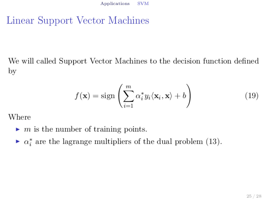
25. Applications SVM Linear Support Vector Machines We will called Support Vector Machines to the decision function defined by f(x) = sign (⟨w, x⟩ + b) = sign ( m ∑ i=1 α∗ i yi⟨xi, x⟩ + b ) (20) Where ▶ m is the number of training points. ▶ α∗ i are the lagrange multipliers of the dual problem (13). 25 / 28
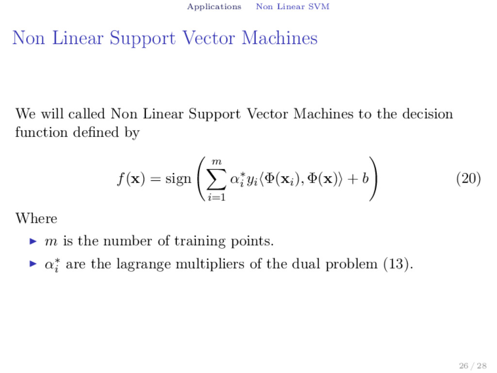
26. Applications Non Linear SVM Non Linear Support Vector Machines We will called Non Linear Support Vector Machines to the decision function defined by f(x) = sign (⟨w, Φ(x)⟩ + b) = sign ( m ∑ i=1 α∗ i yi⟨Φ(xi), Φ(x)⟩ + b ) (21) Where ▶ m is the number of training points. ▶ α∗ i are the lagrange multipliers of the dual problem (13). 26 / 28
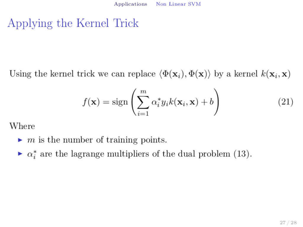
27. Applications Non Linear SVM Applying the Kernel Trick Using the kernel trick we can replace ⟨Φ(xi), Φ(x)⟩ by a kernel k(xi, x) f(x) = sign ( m ∑ i=1 α∗ i yik(xi, x) + b ) (22) Where ▶ m is the number of training points. ▶ α∗ i are the lagrange multipliers of the dual problem (13). 27 / 28
28. Applications Non Linear SVM References for Support Vector Machines [31] Mehryar Mohri, Afshin Rostamizadeh, and Ameet Talwalkar. Foundations of Machine Learning. The MIT Press, 2012. 28 / 28