Sholom Schechtman

(Télécom SudParis)

Title — The late-stage training dynamics of (stochastic) subgradient descent on homogeneous neural networks

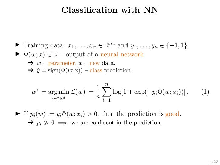
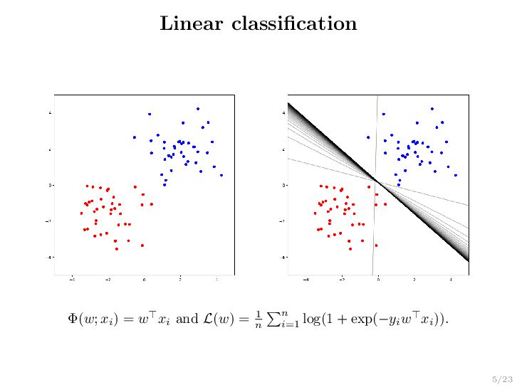
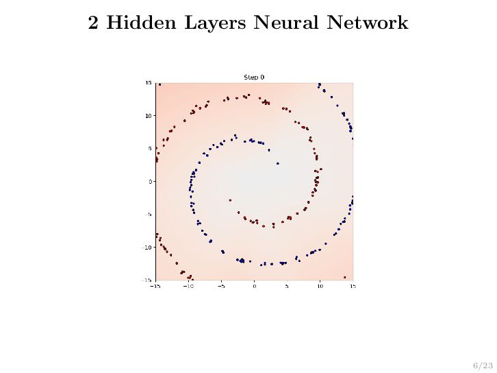
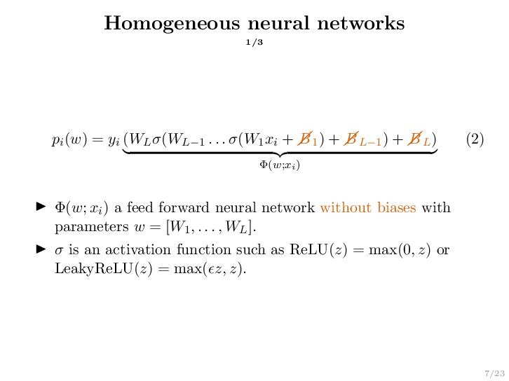
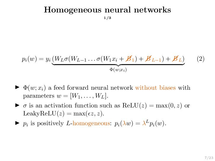
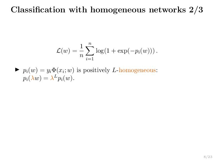
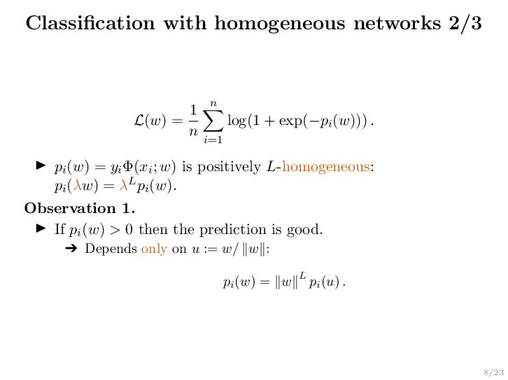
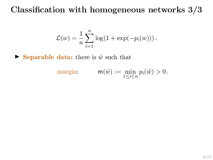
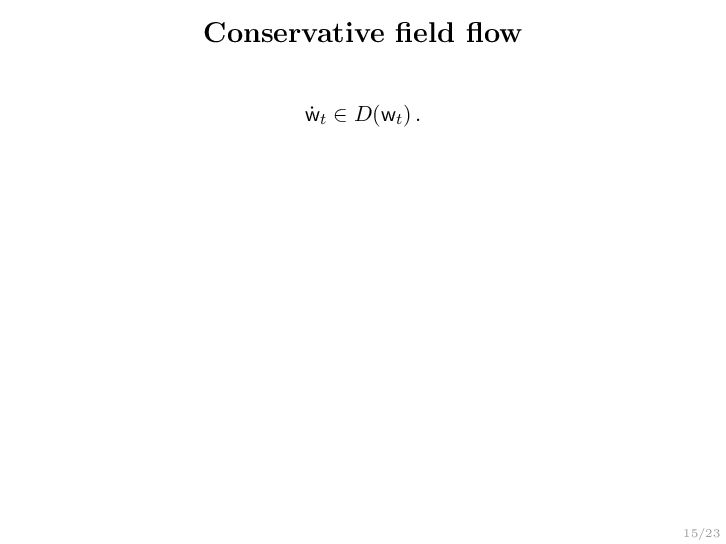
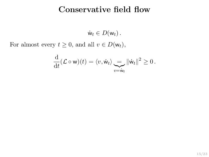
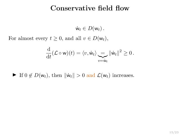
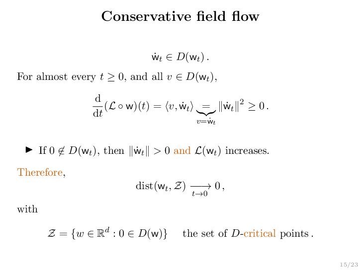
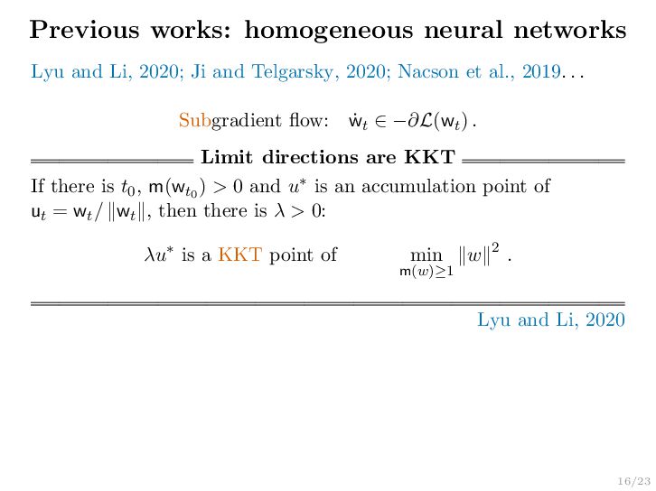
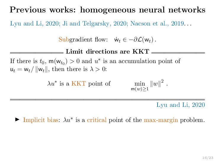
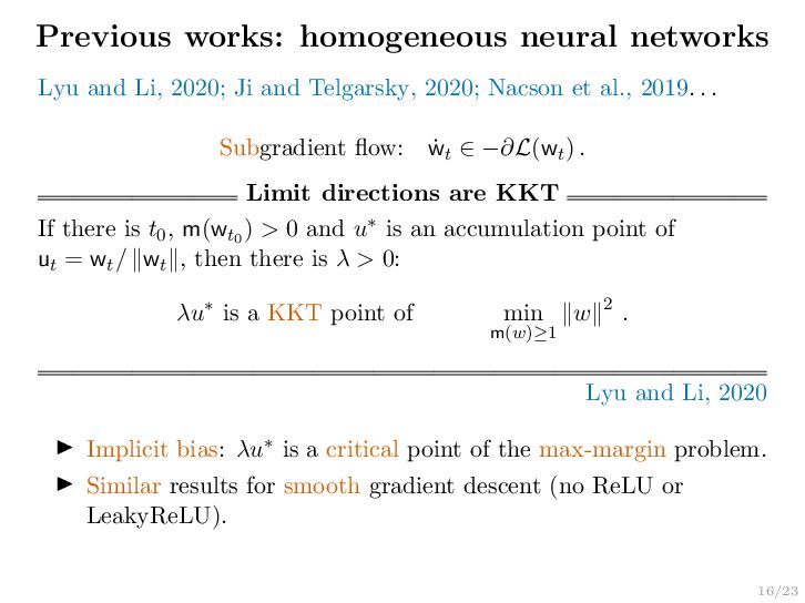
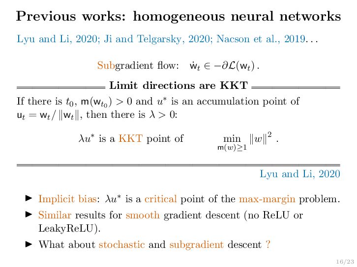
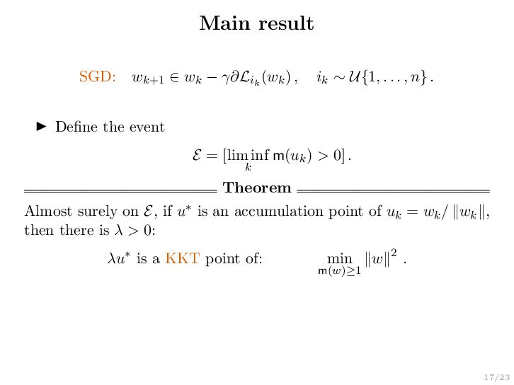
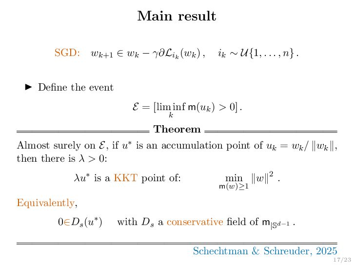
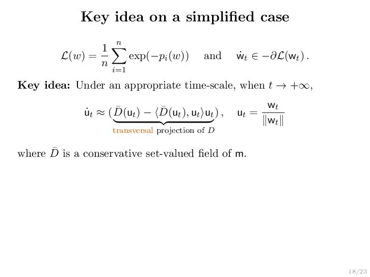
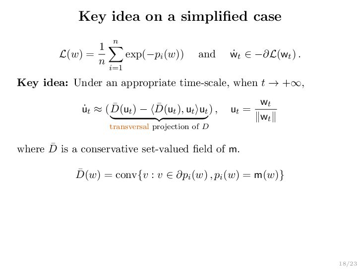
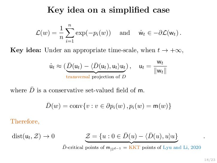
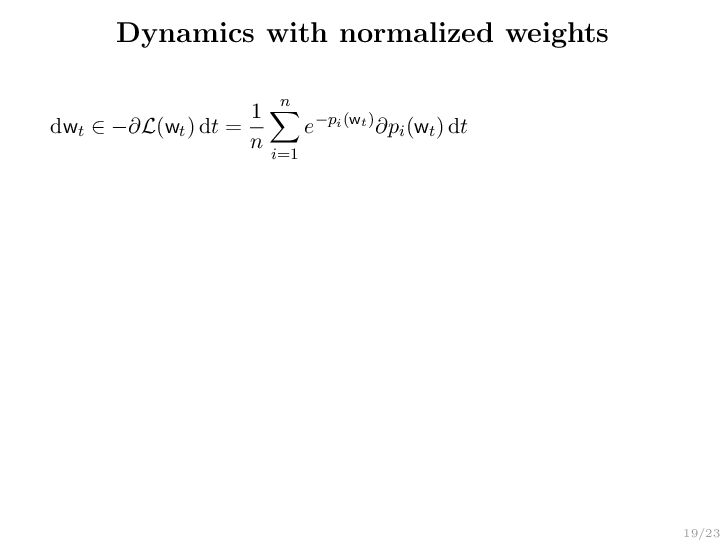
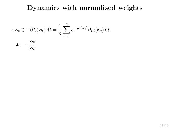
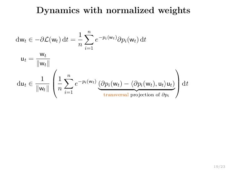
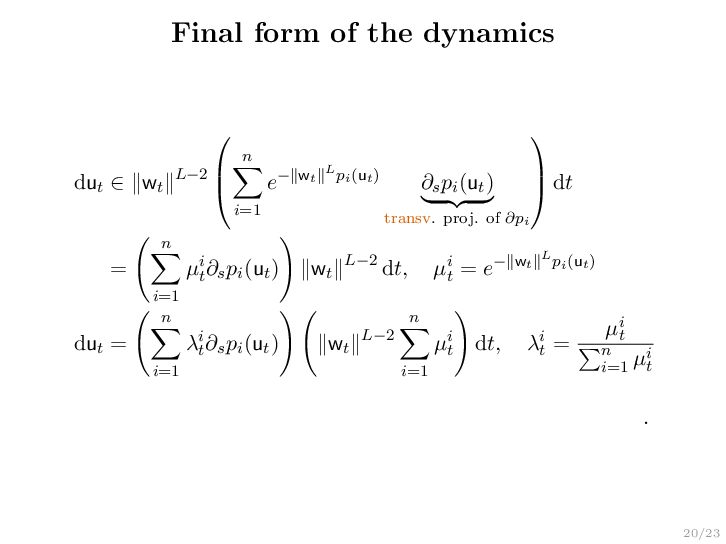
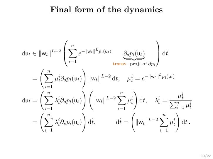
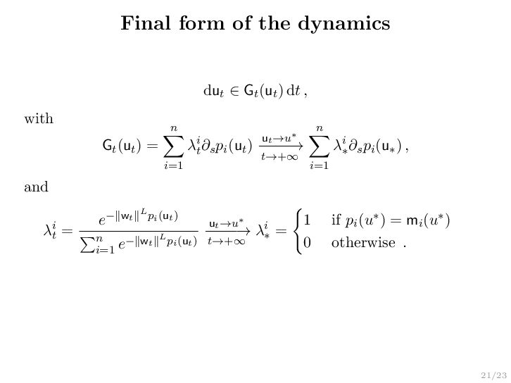
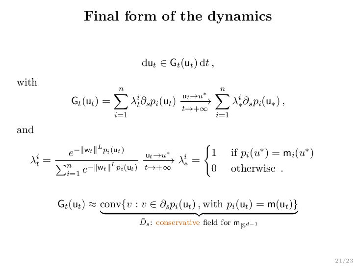
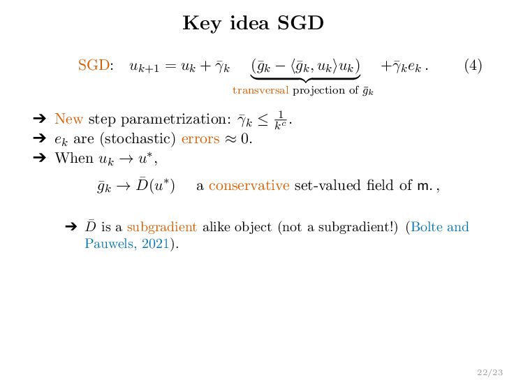
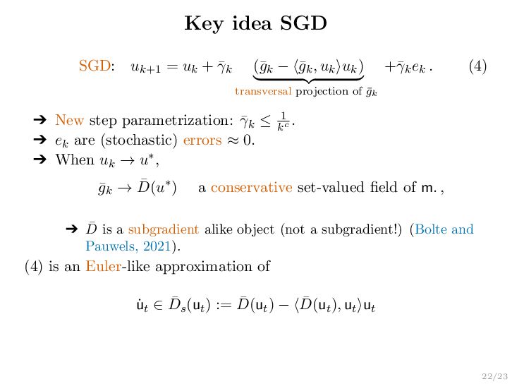
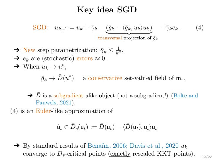
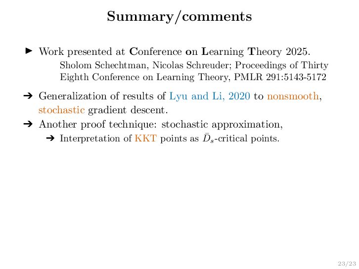
Abstract — We analyze the implicit bias of constant step stochastic subgradient descent (SGD). We consider the setting of binary classification with homogeneous neural networks – a large class of deep neural networks with ReLu-type activation functions such as MLPs and CNNs without biases. Interpreting the dynamics of normalized SGD iterates as an Euler-like discretization of a conservative field flow that is naturally associated to the normalized classification margin, we show that normalized SGD iterates converge to the set of critical points of the normalized margin at late-stage training (i.e., assuming that the data is correctly classified with positive normalized margin). Up to our knowledge, this is the first extension of the analysis of Lyu and Li (2020) on the discrete dynamics of gradient descent to the nonsmooth and stochastic setting. Our main result applies to binary classification with exponential or logistic losses. We additionally discuss extensions to more general settings.

Transcript

1. 1/23 The late-stage training dynamics of SGD on homogeneous neural networks Sholom Schechtman Joint work with Nicolas Schreuder (CNRS, LIGM, Univ. Gustave Eiffel)
2. 2/23 Introduction Modern neural networks are typically overparametrized. ▶ Number of parameters is much larger than the number of data points.
3. 2/23 Introduction Modern neural networks are typically overparametrized. ▶ Number of parameters is much larger than the number of data points. ▶ If a solution exists it is typically not unique.
4. 2/23 Introduction Modern neural networks are typically overparametrized. ▶ Number of parameters is much larger than the number of data points. ▶ If a solution exists it is typically not unique. ➔ However: solution found by (S)GD often generalizes well to unseen data.
5. 2/23 Introduction Modern neural networks are typically overparametrized. ▶ Number of parameters is much larger than the number of data points. ▶ If a solution exists it is typically not unique. ➔ However: solution found by (S)GD often generalizes well to unseen data. Implicit bias hypothesis: ➔ The choice of an algorithm (or/and loss function) induce a solution with good generalization.
6. 3/23 Linear classification Linear prediction with logistic loss – gradient descent training
7. 4/23 Classification with NN ▶ Training data: x1, . . . , xn ∈ Rnx and y1, . . . , yn ∈ {−1, 1}.
8. 4/23 Classification with NN ▶ Training data: x1, . . . , xn ∈ Rnx and y1, . . . , yn ∈ {−1, 1}. ▶ Φ(w; x) ∈ R – output of a neural network ➔ w – parameter, x – new data. ➔ ˆ y = sign(Φ(w; x)) – class prediction.
9. 4/23 Classification with NN ▶ Training data: x1, . . . , xn ∈ Rnx and y1, . . . , yn ∈ {−1, 1}. ▶ Φ(w; x) ∈ R – output of a neural network ➔ w – parameter, x – new data. ➔ ˆ y = sign(Φ(w; x)) – class prediction. w∗ = arg min w∈Rd L(w) := 1 n n i=1 log[1 + exp(−yiΦ(w; xi))] . (1) ▶ If pi(w) := yiΦ(w; xi) > 0, then the prediction is good. ➔ pi ≫ 0 =⇒ we are confident in the prediction.
10. 5/23 Linear classification Φ(w; xi ) = w⊤xi and L(w) = 1 n n i=1 log(1 + exp(−yi w⊤xi )).
11. 6/23 2 Hidden Layers Neural Network
12. 7/23 Homogeneous neural networks 1/3 pi(w) = yi (WLσ(WL−1 . . . σ(W1xi + B1) + BL−1) + BL) Φ(w;xi) (2) ▶ Φ(w; xi) a feed forward neural network without biases with parameters w = [W1, . . . , WL]. ▶ σ is an activation function such as ReLU(z) = max(0, z) or LeakyReLU(z) = max(ϵz, z).
13. 7/23 Homogeneous neural networks 1/3 pi(w) = yi (WLσ(WL−1 . . . σ(W1xi + B1) + BL−1) + BL) Φ(w;xi) (2) ▶ Φ(w; xi) a feed forward neural network without biases with parameters w = [W1, . . . , WL]. ▶ σ is an activation function such as ReLU(z) = max(0, z) or LeakyReLU(z) = max(ϵz, z). ▶ pi is positively L-homogeneous: pi(λw) = λLpi(w).
14. 8/23 Classification with homogeneous networks 2/3 L(w) = 1 n n i=1 log(1 + exp(−pi(w))) . ▶ pi(w) = yiΦ(xi; w) is positively L-homogeneous: pi(λw) = λLpi(w).
15. 8/23 Classification with homogeneous networks 2/3 L(w) = 1 n n i=1 log(1 + exp(−pi(w))) . ▶ pi(w) = yiΦ(xi; w) is positively L-homogeneous: pi(λw) = λLpi(w). Observation 1. ▶ If pi(w) > 0 then the prediction is good. ➔ Depends only on u := w/ ∥w∥: pi (w) = ∥w∥L pi (u) .
16. 9/23 Classification with homogeneous networks 3/3 L(w) = 1 n n i=1 log(1 + exp(−pi(w))) . ▶ Separable data: there is ˆ w such that margin: m( ˆ w) := min 1≤i≤n pi( ˆ w) > 0 .
17. 9/23 Classification with homogeneous networks 3/3 L(w) = 1 n n i=1 log(1 + exp(−pi(w))) . ▶ Separable data: there is ˆ w such that margin: m( ˆ w) := min 1≤i≤n pi( ˆ w) > 0 . Observation 2. ➔ For λ > 1, L(λ ˆ w) < L( ˆ w): exp(−pi (λ ˆ w)) = exp(−λLpi ( ˆ w)) < exp(−pi ( ˆ w)) .
18. 9/23 Classification with homogeneous networks 3/3 L(w) = 1 n n i=1 log(1 + exp(−pi(w))) . ▶ Separable data: there is ˆ w such that margin: m( ˆ w) := min 1≤i≤n pi( ˆ w) > 0 . Observation 2. ➔ For λ > 1, L(λ ˆ w) < L( ˆ w): exp(−pi (λ ˆ w)) = exp(−λLpi ( ˆ w)) < exp(−pi ( ˆ w)) . ➔ “Optimal” w is such that ∥w∥ → +∞ and L(w) → 0.
19. 9/23 Classification with homogeneous networks 3/3 L(w) = 1 n n i=1 log(1 + exp(−pi(w))) . ▶ Separable data: there is ˆ w such that margin: m( ˆ w) := min 1≤i≤n pi( ˆ w) > 0 . Observation 2. ➔ For λ > 1, L(λ ˆ w) < L( ˆ w): exp(−pi (λ ˆ w)) = exp(−λLpi ( ˆ w)) < exp(−pi ( ˆ w)) . ➔ “Optimal” w is such that ∥w∥ → +∞ and L(w) → 0. Question: What about the “optimal direction” u = w/ ∥w∥ ?
20. 10/23 Previous works: linear classifiers L(w) = 1 n n i=1 log(1 + exp(−yiw⊤xi)) = 1 n n i=1 Li(w) . SGD: wk+1 = wk − γ∇Li(k) (wk) , with ik ∼ U({1, . . . , n}) .
21. 10/23 Previous works: linear classifiers L(w) = 1 n n i=1 log(1 + exp(−yiw⊤xi)) = 1 n n i=1 Li(w) . SGD: wk+1 = wk − γ∇Li(k) (wk) , with ik ∼ U({1, . . . , n}) . Theorem If there is w such that m(w) > 0, then ∥wk∥ → +∞, wk/ ∥wk∥ → u∗ and there is λ > 0, such that λu∗ = arg min m(w)≥1 ∥w∥2 ⇐⇒ u∗ = arg max ∥u∥=1 m(u) Soudry et al., 2018; Nacson et al., 2019 Question: What about homogeneous and nonsmooth NNs?
22. 11/23 Digression on subgradients
23. 12/23 Clarke subgradient Given a locally Lipschitz function L : Rd → R, ∂L(w) := conv{v ∈ Rd : there is wk → w and ∇L(wk) → v} . L(w) = |w|, ∂L(0) = [−1, 1]
24. 12/23 Clarke subgradient Given a locally Lipschitz function L : Rd → R, ∂L(w) := conv{v ∈ Rd : there is wk → w and ∇L(wk) → v} . L(w) = |w|, ∂L(0) = [−1, 1] ▶ Generally not a stable operation ∂g ◦ L ̸= ∂g × ∂L , and ∂(L1 + L2) ̸= ∂L1 + ∂L2 .
25. 13/23 Conservative set-valued fields DL : Rd ⇒ Rd is a conservative field (Bolte and Pauwels, 2021) if: ▶ For every a.c. curve w : R+ → Rd, for a.e. t ≥ 0, d dt (L ◦ w)(t) = ⟨v, ˙ wt⟩ , for all v ∈ D(wt) . (3) Examples: ▶ If L is C1, {∇L} is conservative.
26. 13/23 Conservative set-valued fields DL : Rd ⇒ Rd is a conservative field (Bolte and Pauwels, 2021) if: ▶ For every a.c. curve w : R+ → Rd, for a.e. t ≥ 0, d dt (L ◦ w)(t) = ⟨v, ˙ wt⟩ , for all v ∈ D(wt) . (3) Examples: ▶ If L is C1, {∇L} is conservative. ▶ For most functions in optimization (e.g. semialgebraic) ∂L is conservative.
27. 13/23 Conservative set-valued fields DL : Rd ⇒ Rd is a conservative field (Bolte and Pauwels, 2021) if: ▶ For every a.c. curve w : R+ → Rd, for a.e. t ≥ 0, d dt (L ◦ w)(t) = ⟨v, ˙ wt⟩ , for all v ∈ D(wt) . (3) Examples: ▶ If L is C1, {∇L} is conservative. ▶ For most functions in optimization (e.g. semialgebraic) ∂L is conservative. ▶ For semialgebraic functions, ∂g × ∂L and ∂L1 + ∂L2 are conservative.
28. 14/23 Conservative field of m(w) If, m(w) = min i pi(w) , with pi semialgebraic, then ¯ D(w) = conv{v : v ∈ ∂pi(w) , with pi(w) = m(w)} is a conservative field of m(w) (generally not a subgradient!)
29. 15/23 Conservative field flow ˙ wt ∈ D(wt) .
30. 15/23 Conservative field flow ˙ wt ∈ D(wt) . For almost every t ≥ 0, and all v ∈ D(wt), d dt (L ◦ w)(t) = ⟨v, ˙ wt⟩ = v= ˙ wt ∥ ˙ wt∥2 ≥ 0 .
31. 15/23 Conservative field flow ˙ wt ∈ D(wt) . For almost every t ≥ 0, and all v ∈ D(wt), d dt (L ◦ w)(t) = ⟨v, ˙ wt⟩ = v= ˙ wt ∥ ˙ wt∥2 ≥ 0 . ▶ If 0 ̸∈ D(wt), then ∥ ˙ wt∥ > 0 and L(wt) increases.
32. 15/23 Conservative field flow ˙ wt ∈ D(wt) . For almost every t ≥ 0, and all v ∈ D(wt), d dt (L ◦ w)(t) = ⟨v, ˙ wt⟩ = v= ˙ wt ∥ ˙ wt∥2 ≥ 0 . ▶ If 0 ̸∈ D(wt), then ∥ ˙ wt∥ > 0 and L(wt) increases. Therefore, dist(wt, Z) − −→ t→0 0 , with Z = {w ∈ Rd : 0 ∈ D(w)} the set of D-critical points .
33. 16/23 Previous works: homogeneous neural networks Lyu and Li, 2020; Ji and Telgarsky, 2020; Nacson et al., 2019. . . Subgradient flow: ˙ wt ∈ −∂L(wt) . Limit directions are KKT If there is t0, m(wt0 ) > 0 and u∗ is an accumulation point of ut = wt/ ∥wt∥, then there is λ > 0: λu∗ is a KKT point of min m(w)≥1 ∥w∥2 . Lyu and Li, 2020
34. 16/23 Previous works: homogeneous neural networks Lyu and Li, 2020; Ji and Telgarsky, 2020; Nacson et al., 2019. . . Subgradient flow: ˙ wt ∈ −∂L(wt) . Limit directions are KKT If there is t0, m(wt0 ) > 0 and u∗ is an accumulation point of ut = wt/ ∥wt∥, then there is λ > 0: λu∗ is a KKT point of min m(w)≥1 ∥w∥2 . Lyu and Li, 2020 ▶ Implicit bias: λu∗ is a critical point of the max-margin problem.
35. 16/23 Previous works: homogeneous neural networks Lyu and Li, 2020; Ji and Telgarsky, 2020; Nacson et al., 2019. . . Subgradient flow: ˙ wt ∈ −∂L(wt) . Limit directions are KKT If there is t0, m(wt0 ) > 0 and u∗ is an accumulation point of ut = wt/ ∥wt∥, then there is λ > 0: λu∗ is a KKT point of min m(w)≥1 ∥w∥2 . Lyu and Li, 2020 ▶ Implicit bias: λu∗ is a critical point of the max-margin problem. ▶ Similar results for smooth gradient descent (no ReLU or LeakyReLU).
36. 16/23 Previous works: homogeneous neural networks Lyu and Li, 2020; Ji and Telgarsky, 2020; Nacson et al., 2019. . . Subgradient flow: ˙ wt ∈ −∂L(wt) . Limit directions are KKT If there is t0, m(wt0 ) > 0 and u∗ is an accumulation point of ut = wt/ ∥wt∥, then there is λ > 0: λu∗ is a KKT point of min m(w)≥1 ∥w∥2 . Lyu and Li, 2020 ▶ Implicit bias: λu∗ is a critical point of the max-margin problem. ▶ Similar results for smooth gradient descent (no ReLU or LeakyReLU). ▶ What about stochastic and subgradient descent ?
37. 17/23 Main result SGD: wk+1 ∈ wk − γ∂Lik (wk) , ik ∼ U{1, . . . , n} . ▶ Define the event E = [lim inf k m(uk) > 0] . Theorem Almost surely on E, if u∗ is an accumulation point of uk = wk/ ∥wk∥, then there is λ > 0: λu∗ is a KKT point of: min m(w)≥1 ∥w∥2 .
38. 17/23 Main result SGD: wk+1 ∈ wk − γ∂Lik (wk) , ik ∼ U{1, . . . , n} . ▶ Define the event E = [lim inf k m(uk) > 0] . Theorem Almost surely on E, if u∗ is an accumulation point of uk = wk/ ∥wk∥, then there is λ > 0: λu∗ is a KKT point of: min m(w)≥1 ∥w∥2 . Equivalently, 0∈Ds(u∗) with Ds a conservative field of m|Sd−1 . Schechtman & Schreuder, 2025
39. 18/23 Key idea on a simplified case L(w) = 1 n n i=1 exp(−pi(w)) and ˙ wt ∈ −∂L(wt) . Key idea: Under an appropriate time-scale, when t → +∞, ˙ ut ≈ ( ¯ D(ut) − ⟨ ¯ D(ut), ut⟩ut transversal projection of D ) , ut = wt ∥wt∥ where ¯ D is a conservative set-valued field of m.
40. 18/23 Key idea on a simplified case L(w) = 1 n n i=1 exp(−pi(w)) and ˙ wt ∈ −∂L(wt) . Key idea: Under an appropriate time-scale, when t → +∞, ˙ ut ≈ ( ¯ D(ut) − ⟨ ¯ D(ut), ut⟩ut transversal projection of D ) , ut = wt ∥wt∥ where ¯ D is a conservative set-valued field of m. ¯ D(w) = conv{v : v ∈ ∂pi(w) , pi(w) = m(w)}
41. 18/23 Key idea on a simplified case L(w) = 1 n n i=1 exp(−pi(w)) and ˙ wt ∈ −∂L(wt) . Key idea: Under an appropriate time-scale, when t → +∞, ˙ ut ≈ ( ¯ D(ut) − ⟨ ¯ D(ut), ut⟩ut transversal projection of D ) , ut = wt ∥wt∥ where ¯ D is a conservative set-valued field of m. ¯ D(w) = conv{v : v ∈ ∂pi(w) , pi(w) = m(w)} Therefore, dist(ut, Z) → 0 Z = {u : 0 ∈ ¯ D(u) − ⟨ ¯ D(u), u⟩u} ¯ D-critical points of m|Sd−1 = KKT points of Lyu and Li, 2020 .
42. 19/23 Dynamics with normalized weights dwt ∈ −∂L(wt) dt = 1 n n i=1 e−pi(wt)∂pi(wt) dt
43. 19/23 Dynamics with normalized weights dwt ∈ −∂L(wt) dt = 1 n n i=1 e−pi(wt)∂pi(wt) dt ut = wt ∥wt∥
44. 19/23 Dynamics with normalized weights dwt ∈ −∂L(wt) dt = 1 n n i=1 e−pi(wt)∂pi(wt) dt ut = wt ∥wt∥ dut ∈ 1 ∥wt∥    1 n n i=1 e−pi(wt) (∂pi(wt) − ⟨∂pi(wt), ut⟩ut) transversal projection of ∂pi    dt
45. 19/23 Dynamics with normalized weights dwt ∈ −∂L(wt) dt = 1 n n i=1 e−pi(wt)∂pi(wt) dt ut = wt ∥wt∥ dut ∈ 1 ∥wt∥    1 n n i=1 e−pi(wt) (∂pi(wt) − ⟨∂pi(wt), ut⟩ut) transversal projection of ∂pi    dt = ∥wt∥L−1 ∥wt∥    1 n n i=1 e−∥wt∥Lpi(ut) (∂pi(ut) − ⟨∂pi(ut), ut⟩ut) transversal projection of ∂pi    dt
46. 19/23 Dynamics with normalized weights dwt ∈ −∂L(wt) dt = 1 n n i=1 e−pi(wt)∂pi(wt) dt ut = wt ∥wt∥ dut ∈ 1 ∥wt∥    1 n n i=1 e−pi(wt) (∂pi(wt) − ⟨∂pi(wt), ut⟩ut) transversal projection of ∂pi    dt = ∥wt∥L−1 ∥wt∥    1 n n i=1 e−∥wt∥Lpi(ut) (∂pi(ut) − ⟨∂pi(ut), ut⟩ut) transversal projection of ∂pi    dt = ∥wt∥L−2    n i=1 e−∥wt∥Lpi(ut) ∂spi(ut) transv. proj. of ∂pi    dt
47. 20/23 Final form of the dynamics dut ∈ ∥wt∥L−2    n i=1 e−∥wt∥Lpi(ut) ∂spi(ut) transv. proj. of ∂pi    dt .
48. 20/23 Final form of the dynamics dut ∈ ∥wt∥L−2    n i=1 e−∥wt∥Lpi(ut) ∂spi(ut) transv. proj. of ∂pi    dt = n i=1 µi t ∂spi(ut) ∥wt∥L−2 dt, µi t = e−∥wt∥Lpi(ut) .
49. 20/23 Final form of the dynamics dut ∈ ∥wt∥L−2    n i=1 e−∥wt∥Lpi(ut) ∂spi(ut) transv. proj. of ∂pi    dt = n i=1 µi t ∂spi(ut) ∥wt∥L−2 dt, µi t = e−∥wt∥Lpi(ut) dut = n i=1 λi t ∂spi(ut) ∥wt∥L−2 n i=1 µi t dt, λi t = µi t n i=1 µi t .
50. 20/23 Final form of the dynamics dut ∈ ∥wt∥L−2    n i=1 e−∥wt∥Lpi(ut) ∂spi(ut) transv. proj. of ∂pi    dt = n i=1 µi t ∂spi(ut) ∥wt∥L−2 dt, µi t = e−∥wt∥Lpi(ut) dut = n i=1 λi t ∂spi(ut) ∥wt∥L−2 n i=1 µi t dt, λi t = µi t n i=1 µi t = n i=1 λi t ∂spi(ut) d˜ t, d˜ t = ∥wt∥L−2 n i=1 µi t dt .
51. 21/23 Final form of the dynamics dut ∈ Gt(ut) dt , with Gt(ut) = n i=1 λi t ∂spi(ut) ut→u∗ − − − −→ t→+∞ n i=1 λi ∗ ∂spi(u∗) , and λi t = e−∥wt∥Lpi(ut) n i=1 e−∥wt∥Lpi(ut) ut→u∗ − − − −→ t→+∞ λi ∗ = 1 if pi(u∗) = mi(u∗) 0 otherwise .
52. 21/23 Final form of the dynamics dut ∈ Gt(ut) dt , with Gt(ut) = n i=1 λi t ∂spi(ut) ut→u∗ − − − −→ t→+∞ n i=1 λi ∗ ∂spi(u∗) , and λi t = e−∥wt∥Lpi(ut) n i=1 e−∥wt∥Lpi(ut) ut→u∗ − − − −→ t→+∞ λi ∗ = 1 if pi(u∗) = mi(u∗) 0 otherwise . Gt(ut) ≈ conv{v : v ∈ ∂spi(ut) , with pi(ut) = m(ut)} ¯ Ds: conservative field for m|Sd−1
53. 22/23 Key idea SGD SGD: uk+1 = uk + ¯ γk (¯ gk − ⟨¯ gk, uk⟩uk) transversal projection of ¯ gk +¯ γkek . (4) ➔ New step parametrization: ¯ γk ≤ 1 kc . ➔ ek are (stochastic) errors ≈ 0. ➔ When uk → u∗, ¯ gk → ¯ D(u∗) a conservative set-valued field of m. , ➔ ¯ D is a subgradient alike object (not a subgradient!) (Bolte and Pauwels, 2021).
54. 22/23 Key idea SGD SGD: uk+1 = uk + ¯ γk (¯ gk − ⟨¯ gk, uk⟩uk) transversal projection of ¯ gk +¯ γkek . (4) ➔ New step parametrization: ¯ γk ≤ 1 kc . ➔ ek are (stochastic) errors ≈ 0. ➔ When uk → u∗, ¯ gk → ¯ D(u∗) a conservative set-valued field of m. , ➔ ¯ D is a subgradient alike object (not a subgradient!) (Bolte and Pauwels, 2021). (4) is an Euler-like approximation of ˙ ut ∈ ¯ Ds(ut) := ¯ D(ut) − ⟨ ¯ D(ut), ut⟩ut
55. 22/23 Key idea SGD SGD: uk+1 = uk + ¯ γk (¯ gk − ⟨¯ gk, uk⟩uk) transversal projection of ¯ gk +¯ γkek . (4) ➔ New step parametrization: ¯ γk ≤ 1 kc . ➔ ek are (stochastic) errors ≈ 0. ➔ When uk → u∗, ¯ gk → ¯ D(u∗) a conservative set-valued field of m. , ➔ ¯ D is a subgradient alike object (not a subgradient!) (Bolte and Pauwels, 2021). (4) is an Euler-like approximation of ˙ ut ∈ ¯ Ds(ut) := ¯ D(ut) − ⟨ ¯ D(ut), ut⟩ut ➔ By standard results of Bena¨ ım, 2006; Davis et al., 2020 uk converge to ¯ Ds-critical points (exactly rescaled KKT points).
56. 23/23 Summary/comments ▶ Work presented at Conference on Learning Theory 2025. Sholom Schechtman, Nicolas Schreuder; Proceedings of Thirty Eighth Conference on Learning Theory, PMLR 291:5143-5172
57. 23/23 Summary/comments ▶ Work presented at Conference on Learning Theory 2025. Sholom Schechtman, Nicolas Schreuder; Proceedings of Thirty Eighth Conference on Learning Theory, PMLR 291:5143-5172 ➔ Generalization of results of Lyu and Li, 2020 to nonsmooth, stochastic gradient descent. ➔ Another proof technique: stochastic approximation, ➔ Interpretation of KKT points as ¯ Ds -critical points.
58. 23/23 Summary/comments ▶ Work presented at Conference on Learning Theory 2025. Sholom Schechtman, Nicolas Schreuder; Proceedings of Thirty Eighth Conference on Learning Theory, PMLR 291:5143-5172 ➔ Generalization of results of Lyu and Li, 2020 to nonsmooth, stochastic gradient descent. ➔ Another proof technique: stochastic approximation, ➔ Interpretation of KKT points as ¯ Ds -critical points. Comments. ▶ Convergence under constant stepsize : γ constant but effective stepsize ¯ γk → 0.
59. 23/23 Summary/comments ▶ Work presented at Conference on Learning Theory 2025. Sholom Schechtman, Nicolas Schreuder; Proceedings of Thirty Eighth Conference on Learning Theory, PMLR 291:5143-5172 ➔ Generalization of results of Lyu and Li, 2020 to nonsmooth, stochastic gradient descent. ➔ Another proof technique: stochastic approximation, ➔ Interpretation of KKT points as ¯ Ds -critical points. Comments. ▶ Convergence under constant stepsize : γ constant but effective stepsize ¯ γk → 0. ▶ (Hopefully) proof technique adapts to algorithms others than SGD.
60. 23/23 Summary/comments ▶ Work presented at Conference on Learning Theory 2025. Sholom Schechtman, Nicolas Schreuder; Proceedings of Thirty Eighth Conference on Learning Theory, PMLR 291:5143-5172 ➔ Generalization of results of Lyu and Li, 2020 to nonsmooth, stochastic gradient descent. ➔ Another proof technique: stochastic approximation, ➔ Interpretation of KKT points as ¯ Ds -critical points. Comments. ▶ Convergence under constant stepsize : γ constant but effective stepsize ¯ γk → 0. ▶ (Hopefully) proof technique adapts to algorithms others than SGD. ▶ Open question: Neural Network with biases?